Untar the package of C code on the class website named 'fitting.tar'. This will create a subdirectory named 'fitting' under the current directory. Change into that 'fitting' subdirectory.
In this section we will fit some hypothetical experimental data points to a linear function with the least squares method. For learning purposes here we will "cheat" a little and work with data points that have been generated by a C program we will write, but of course in general linear fitting is actually used in practice when we have experimental data that come from some unknown dependence. Begin by opening the source code file generate_data.c in a text editor:
gedit generate_data.c &
This is a short program that generates x and y data point pairs, where x is swept from 0.0 to 10.0 with an increment of 0.1. Note the line that uses the math library call rand(). This will assign a pseudorandom value to the floating point variable r that will lie somewhere between -0.5 and 0.5. With the editor complete the two lines indicated that assign a y coordinate value to each data point and send the x and y values out to standard output in a format that can be scanned by the C fscanf function. Make your y values be the sum of three terms: some constant multiplier times the x coordinate, another constant offset, and the pseudorandom number r. Choose what values you would like for the two arbitrary constants. Save your source code file and compile with:
gcc -Wall generate_data.c -o generate_data -lm
If you run the compiled program './generate_data' you should see x and y coordinate pairs being output to your terminal. Now capture the output into a data file with:
./generate_data >| data.dat
Now build the linear fitting code that has been discussed in lecture with:
gcc -Wall fitlinear_sweep.c fitlinear.c data_file.c -o fitlinear_sweep -lm
Note that we have to link to the source code in fitlinear.c and data_file.c to get the routines for computing the linear fit and reading data files. First try running your compiled executable program and viewing its help line output:
./fitlinear_sweep
Now try solving for a least squares linear fit with your generated data with:
./fitlinear_sweep data.dat 0.0 10.0 1.0 >| fitlinear_sweep.dat
This should write an output data file named fitlinear_sweep.dat that results from sweeping the linear function that has been fit to the data that we artificially generated. What are the starting, stopping and increment values for this sweep? How many sweep evaluation points will this generate in the fitlinear_sweep.dat file? If the intended use of this file is to simply plot in gnuplot, do we need more points generated? What is the minimum number of points that it would make sense to generate with this program if all we want to do is plot the resulting linear relationship?
Now open a second terminal window, change its shell into the fitting subdirectory, and start a gnuplot process. Plot two files together on the same plot, first the raw data points in 'data.dat' in points mode, and the sweep of your generated fitting line in 'fitlinear_sweep.dat' in lines mode. You should end up with something that looks like:
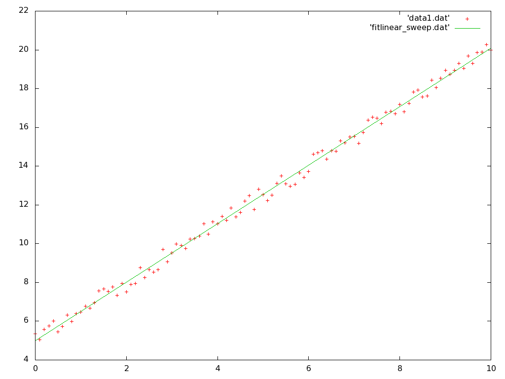
but will probably look different according to your choice of the constants that generated the sample data file.
Now go back to the terminal output when you ran the program that fit the line. You should see two solved linear function coefficients that were output to stderr on the terminal. Are these coefficients consistant with the plot?
Now go back to your editor and try another couple of values for the two constants of choice. Recompile generate_data.c, and rerun it to generate a new set of data points. Rerun the fitlinear_sweep program, and replot in gnuplot to check the difference.
Now in your gnuplot process, plot the supplied data file 'triangle.dat' in the points mode. If you like, you can make the points mode show up better in the plot by adding the parameter 'pointtype 7' to the plot command. Note that this set of data coordinates describes an oscillatory system with a y coordinate that traces out a 'triangle wave'. What is the frequency of oscillation? Also note that the zero x coordinate value does not lie on either the zero crossing of a y or at the peak value of y. We will be fitting this experimental data file to a sum of sinusoids, so this phase means that there will need to be both sine and cosine terms in the fit.
Now build the sinusoidal fitting tools discussed in lecture with:
gcc -Wall fitsine_sweep.c fitsine.c lineq.c data_file.c -o fitsine_sweep -lm
Note that the routines in lineq.c now need to be linked in to solve the system of linear equations that the fit requires. Run the fit with:
./fitsine_sweep triangle.dat 0.0625 0 32 0.01 >| fitsine_sweep.dat
Now add the 'fitsine_sweep.dat' function to your gnuplot so that both the data points and the sinusoidal fit are plotted together. You should end up with something that looks like:
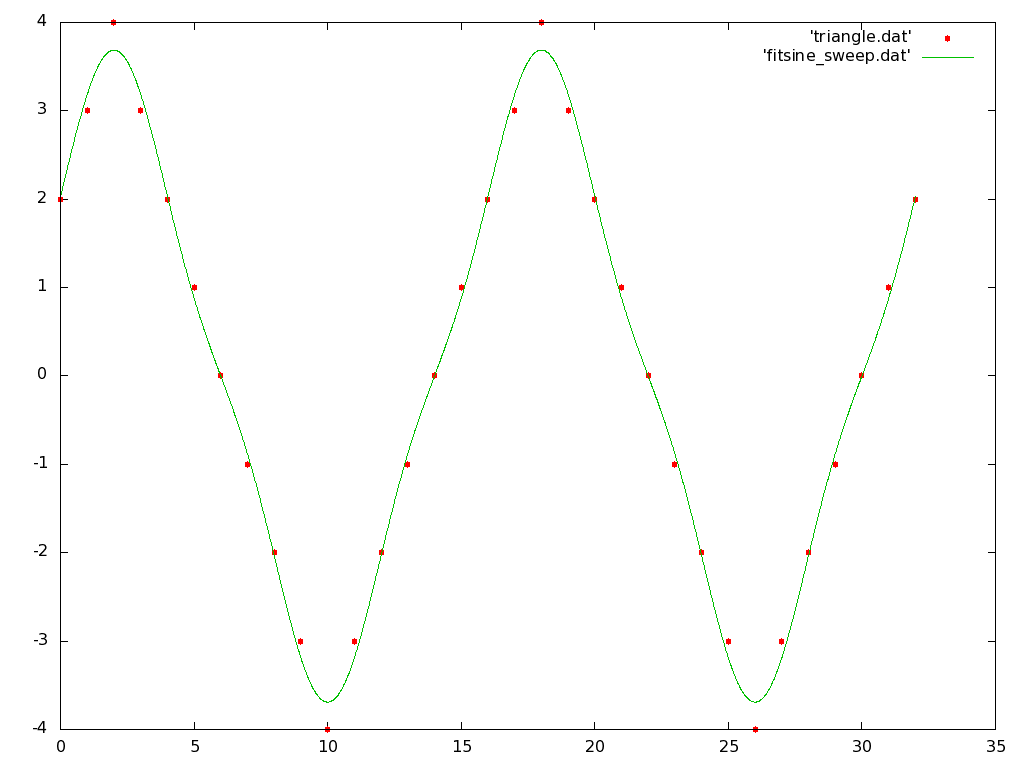
Note that with only three harmonics of sinusoids, the fit routine can come fairly close to a triangle wave. Back in the terminal window where the fit program was run, note the seven coeficient values sent to the stderr stream. What harmonics of sinusoids do each coefficient correspond to? Do these values make sense?