 with μ set to zero and
σ set to 1. Note that the source code already includes the header file
'constants.h', so you may make use of the
constant symbols in that file if you would like.
Save your source code file and compile with:
with μ set to zero and
σ set to 1. Note that the source code already includes the header file
'constants.h', so you may make use of the
constant symbols in that file if you would like.
Save your source code file and compile with:Untar the package of C code on the class website named 'integration.tar'. This will create a subdirectory named 'integration' under the current directory. Change into that 'integration' subdirectory.
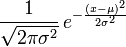
In this section we will integrate the standard normal Gaussian distribution function with both the Trapezoidal and Simpson's Rules. This function has been studied for centuries as one of the fundamental relationships of Statistics. While no analytical integration is possible, the numerical integration of this function has been accurately tabulated. See http://en.wikipedia.org/wiki/Gaussian_distribution for more details.
We will be duplicating the known numerical values of double-sided integration for one, two and three standard deviations that are:
| Integration limits | Numerical value |
|---|---|
| ±1 standard deviation | 0.682689492137 |
| ±2 standard deviation | 0.954499736104 |
| ±3 standard deviation | 0.997300203937 |
Begin by opening the source code file integrate_function.c in a text editor:
gedit integrate_function.c &
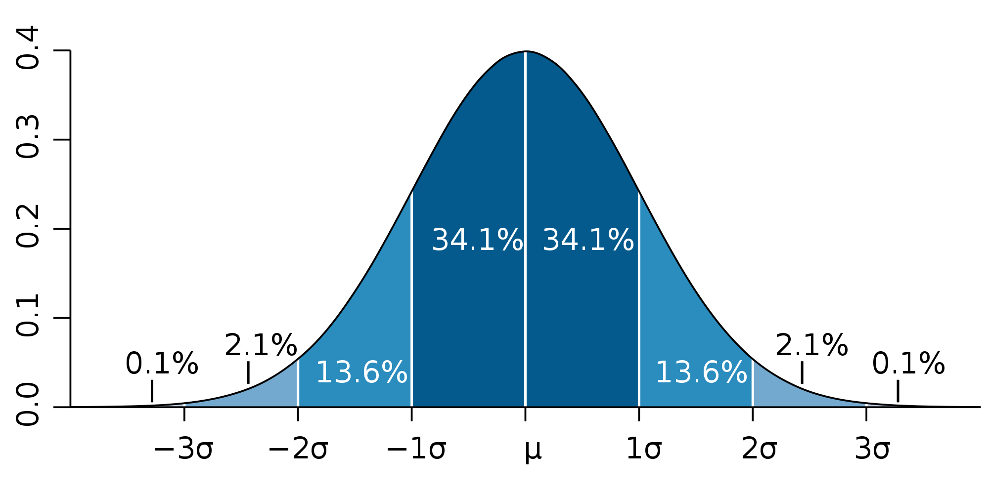
With the editor complete the source code lines indicated so that the
function to be passed to the integration routines is the standard distribution
function with zero mean and unity standard deviation. This function is
with μ set to zero and
σ set to 1. Note that the source code already includes the header file
'constants.h', so you may make use of the
constant symbols in that file if you would like.
Save your source code file and compile with:
gcc -Wall integrate_function.c integrate.c -o integrate_function -lm
Note that we have to link to the source code in integrate.c to get the routine for Trapezoidal and Simpson's Rule integration. First try running your compiled executable program and viewing its help line output:
./integrate_function
What values of Xstart and Xstop for the integration limits correspond to ±1 standard deviation, ±2 standard deviations and ±3 standard deviations? Now try running an integration with a very fine integration time step of 0.001 over ±1 standard deviation. Does the integrated value displayed on standard output correspond with the table value above? Now try ±2 standard deviations and ±3 standard deviations with the same step size.
Since the Trapezoidal Rule has a relatively large error term compared to Simpson's Rule, this program gives us an easy opportunity to study the dependence of error on step size. Use the computer's calculator tool to find the error between the accurate value of the integration for ±1 standard deviation limits in the table above with the value your program calculated with a step size of 0.001. Now if the step size were to be varied by a factor of ten for these integrations, knowing that the Trapezoidal Rule has an error term of order two, what dependence of error on step size would you expect to see? Run integrations with step sizes of 0.01 and 0.1 over ±1 standard deviation limits. Your result from the Simpson's Rule integration should not change much, but you should see increasing errors in the Trapezoidal Rule results. Calculate the two error values between the accurate value above and the two values your program computes at these coarser step sizes. What dependence of error on step size do you observe?
We will now look at the ability of these numerical integration algorithms to negotiate functions with sharp discontinuities. Now go back to your source code edit window and modify your main program so that the function being integrated is a unit step function, that is, the function value is 0 for argument x values less than 0, and the function is 1 for x values greater than or equal to 0. (Hint: you will probably need a C if statement in your function.) Recompile your source code. In the integration problem in section 1 the integrand function was relatively smooth, and we saw that even with a fairly course step size of 0.1, the quadratic polynomial fitting contained in the Simpson algorithm still produced an integration with quite low error. Try running your program with the step function now with a step size of 0.1, running from -1 to 1. What value would you expect from this integration? What errors do both algorithms commit?