Untar the package of C code on the class website named 'interpolation.tar'. This will create a subdirectory named 'interpolation' under the current directory. Change into that 'interpolation' subdirectory.
In this lab we will fit some hypothetical experimental data points to polynomials. For learning purposes here we will "cheat" a little and work with data points that lie on an already known function, in this case cos(2 π x), but of course in general polynomial interpolation is actually used in practice when we have experimental data that come from some unknown dependence. We will see that the curvature of the cosine function fits particularly well to polynomials, as you would expect from the Taylor series approximation for a cosine function. Begin by starting a text editor session in the background with:
gedit &
With the editor create two new files in the current directory named data_cosine3.dat and data_cosine5.dat. In the first file write three text lines in the format that will be scanned by the C fscanf function. The lines should list the x and y coordinates of three data points. The x coordinates are -0.25, 0 and 0.25, and the y coordinates are the values of the function cos(2 π x) at those x values. In the second file do the same except there should be five lines, corresponding to x values of -0.25, -0.125, 0, 0.125 and 0.25. Save both data files.
Now open the source code file interpolate_sweep.c with the text editor. Inspect the conditional compilation lines to find the symbols that should be included in a '-D' option to gcc at compile time so that the program uses either the Lagrange or Newton formulation of the interpolation polynomial. Compile the source code with:
gcc -Wall -Dxxxxx interpolate_sweep.c interpolate.c data_file.c -o interpolate_sweep -lm
where 'xxxxx' in the '-D' argument is replaced by the symbol appropriate for the Newton method. Note that we have to link to the source code in interpolate.c and data_file.c to get the routines for computing the interpolation polynomial and reading data files. First try running your compiled executable program and viewing its help line output:
./interpolate_sweep
Now try an interpolation with the data file containing three data points with:
./interpolate_sweep data_cosine3.dat -0.25 0.25 0.01 >| interpolate_sweep.dat
This should write an output data file named interpolate_sweep.dat that results from sweeping the interpolation polynomial. What are the starting, stopping and increment values for this sweep? How many sweep evaluation points will this generate in the interpolate_sweep.dat file? Since there were three data points used to interpolate this polynomial, what order of polynomial was created?
Now open a second terminal window, change its shell into the interpolation subdirectory, and start a gnuplot process. Plot three files together on the same plot, first the raw data points in 'data_cosine3.dat' in points mode, then the sweep of your generated interpolation polynomial in 'interpolate_sweep.dat' in lines mode, and finally the data file 'data_cosine51.dat' in lines mode. This last file is supplied in the tar file, and is simply a sweep of the original dependency function cos(2 π x) with 51 points. If you like, you can make the points mode show up better in gnuplot by adding the parameter 'pointtype 7' in the plot command in the raw data file section. You should end up with something that looks like:
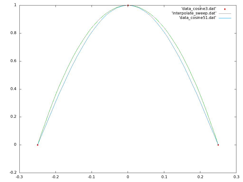
Note that although the interpolated polynomial passes through the three data points as required, this order of polynomial still leaves significant errors with respect to the original data dependence function.
Now go back to the terminal output when you ran the program that interpolated the polynomial. You should see three solved Newton polynomial coefficients that were output to stderr on the terminal. These coefficients are of course applicable for the Newton formulation of the polynomial. Using these three values, write out the Newton polynomial and expand the terms to express the same polynomial in its canonical form, that is, a0 + a1x + a2x². Now compare the coefficients in this formulation with a two term Taylor series approximation to cos(2 π x). Explain the difference.
Now back in your bash shell terminal window, try an interpolation with the data file containing five data points with:
./interpolate_sweep data_cosine5.dat -0.25 0.25 0.01 >| interpolate_sweep.dat
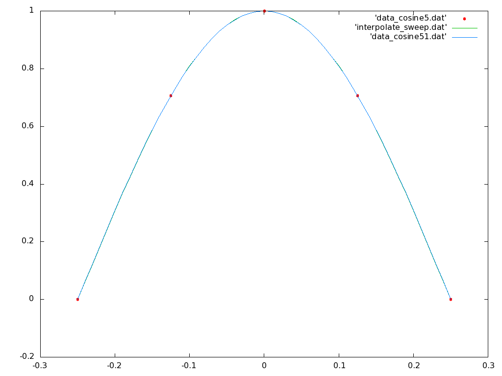
Note that since there were five data points supplied, now there are five coefficients solved for and sent to stderr on the terminal screen. What order polynomial has been interpolated? Go back to the gnuplot terminal window and plot the three files 'data_cosine5.dat', 'interpolate_sweep.dat' and 'data_cosine51.dat' together, the first in points mode with pointtype 7, and the last two in lines mode as before. You should see a much closer interpolation fit that looks like:
Now go back to your terminal window and recompile the source code so that the Lagrange formulation is used to generate the interpolation polynomial. Rerun the program with the five point data file. Replot the generated polynomial in gnuplot.
In this section we will explore fitting polynomials of various orders to a more difficult function, the so-called Runge function. This function is described in section 4.2 of Cheney and Kincaid, and is f(x) = 1/(1+x2). You will see that the curvature of this function makes fitting difficult over a wide range of x values.
First we will prepare a program that calls the sweep.c tool that we used extensively earlier in the semester. Begin by editing a provided source code file with:
gedit runge_sweep.c &
and complete the C code statement indicated in the function 'runge' to allow this program to evaluate the Runge function over a sweep of x values. Compile your code with:
gcc -Wall runge_sweep.c sweep.c -o runge_sweep -lmand observe its help output with:
./runge_sweep
Following the description in our textbook, we will sweep the x value from -5 to +5. Figure what xinc value you will need to evaluate the function at 5, 9, and 101 points. Run the program three times with approprate command lines, and redirect its standard output into the three files 'data_runge5.dat', 'data_runge9.dat' and 'data_runge101.dat', respectively. The first two data files we will use to provide sample points for polynomial interpolation, and the third data file gives a densely sampled picture of the Runge function only for plotting purposes.
As in section I, generate an interpolation with the data file containing five data points with:
./interpolate_sweep data_runge5.dat -5 5 0.01 >| interpolate_sweep.dat
Plot the fit with gnuplot, as in Section I with three plots on one graph, the data points first with points mode, the generated interpolation polynomial next with lines mode, and finally the full resolution Runge function with lines. Your plot should look like:
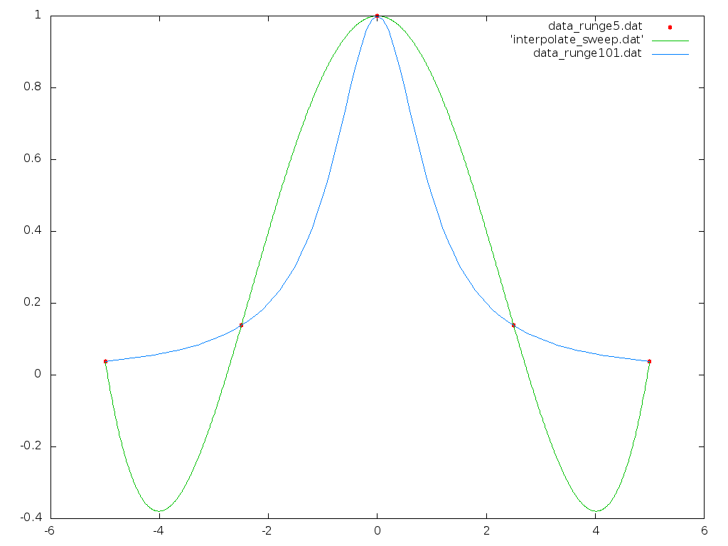
Note that this fit is not particularly close. Although fitting a polynomial over a narrower x range would result in a closer fit, over this wide range from -5 to 5 the curvature of the Runge function doesn't conform to a polynomial shape.
In the case of the cosine function in Section I, using more data points improved the fidelity of the polynomial fit. In an effort to improve the fit to the Runge function, try using the nine point data file with:
./interpolate_sweep data_runge9.dat -5 5 0.01 >| interpolate_sweep.dat
and update the gnuplot. Is the fit better or worse?