Untar the package of C code on the class website named 'montecarlo.tar'. This will create a subdirectory named 'montecarlo' under the current directory. Change into that 'montecarlo' subdirectory.
In this section we will approximate the value of π with the Monte Carlo method. We will generate a number of random two dimensional coordinates within the square defined by -1 < x < 1 and -1 < y < 1, and count the number that end up within a unit circle contained in that square. The process is illustrated by this figure, with the green dots being the "hits" that we will keep track of, and the red dots the trials that we will discard:
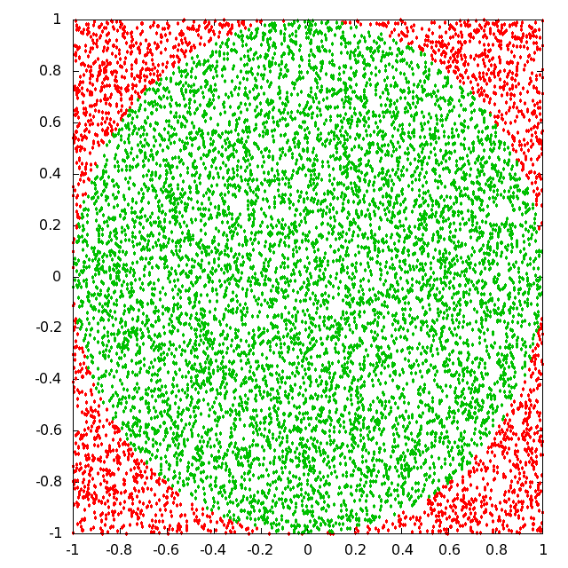
Then the value of π may be measured by the ratio of the areas that is approximated by the ratio of the number of hits inside the circle to the total number of trials. Begin by opening the source code file pi.c in a text editor:
gedit pi.c &
Follow the code as it extracts two integer parameters off of the command line, the first being the total count of random trials to conduct, and the second the integer seed value for the random number generator. For reference, open the file random.c in another window in the gedit text editor to see the two functions in this random number generator utility. Note that the code in pi.c already is set up to seed the generator with a call to random_seed() and set up an iterative loop over all the random trials. Also note the lines of code at the end that calculate the estimate of π from the hit ratio and report a value.
Knowing that the random_gen() function returns a pseudorandom floating point number within the range 0.0 to 1.0, with the editor complete the source code lines inside the main trial loop indicated to generate two random coordinates within the range of the square. Also complete the if statement at the end of the loop so that the variable n_hits is incremented only if the generated coordinates are within the unit circle. Significant computation time can be saved with the observation that a call to sqrt() is not actually needed for this test. Save your source code file and compile with:
gcc -Wall pi.c random.c -o pi -lm
Note that we have to link to the source code in random.c to get the routines for seeding and generating pseudorandom numbers. First try running your compiled executable program and viewing its help line output:
./pi
Now try running a fairly low number of trials, say 1000, with a seed value of 1 and note the value of π this generates. Try different seed values, such as 2, 3, 123456, or any integer value you'd like to try. With only 1000 trials, which of these seed values gives the estimate of π with the least error? Now go back to a seed value of 1 and try increasing the number of random trials to 10000, 100000, 1000000 and 10000000 and note the decreasing error in the estimate. With this last large number of trials, now try different seed values as before and find which one gives the least error.
In this section we will simulate a random walk with the Monte Carlo method. Begin by opening the source code file walk.c in a text editor:
gedit walk.c &
Complete the source code lines indicated to implement the algorithm to propagate the x and y coordinates through a random walk. The method for randomly finding Δx and Δy on the unit circle is:
Set Δx to a pseudorandom number between -1 and +1
Set Δy to a pseudorandom number between -1 and +1
Calculate the radius r = √ Δx2 + Δy2
If the radius is greater than 1, discard the Δx and Δy and generate another pair
Otherwise adjust Δx and Δy by dividing each by the radius
Save your source code file and compile with:
gcc -Wall walk.c random.c -o walk -lm
First try running your compiled executable program and viewing its help line output:
./walk
Then rerun the program with 100 steps with a random seed of your choice. This should generate two data files in the current directory, named walk_position.dat and walk_distance.dat. The first file lists the x and y coordinates of the particle along its walk, and the second file lists the cumulative distance traveled as a function of time.
Start another terminal window, change to the montecarlo directory, and start a gnuplot process. First use gnuplot to display the path of the walk by plotting the walk_position.dat file with lines. Back in the terminal running the bash shell, rerun the program with a few different seed values, which will generate new versions of walk_position.dat and walk_distance.dat. Replot these new paths in the gnuplot window with the 'replot' command.
Now use gnuplot to plot the cumulative distance data in walk_distance.dat. Try running the same random walks with the same seed values you used before and observe how the total distance walked changes significantly. Then try running a few walks with a large number of steps, and replotting walk_distance.dat in gnuplot. How closely do these plots adhere to the theoretical projection that the traveled distance should be the square root of the number of steps?