| Launch velocity: | 100.0 | |
| Launch angle: | 45.0 | |
| Drag coefficient α: | 1.0000e-6 |
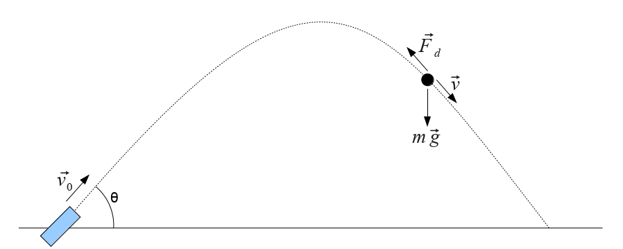
One of the first applications of scientific digital computing technology was predicting ballistic trajectories during World War II. A simplied version of the physical system is shown here. A projectile is launched with an initial velocity v⃗0 and angle θ relative to horizontal, and is subjected to gravitational and drag forces as it flies through the air to its landing point.
In the absence of air drag, the trajectory is a solution of a trivial differential equation accounting for only the uniform downward gravitational field and follows a parabolic path. However, with some realistic models for the drag forces at high velocities, the differential equation becomes significantly nonlinear, and must be solved with numerical methods.
A simple model for the drag force vector F⃗d on an object with velocity v⃗ through a fluid is usually expressed as
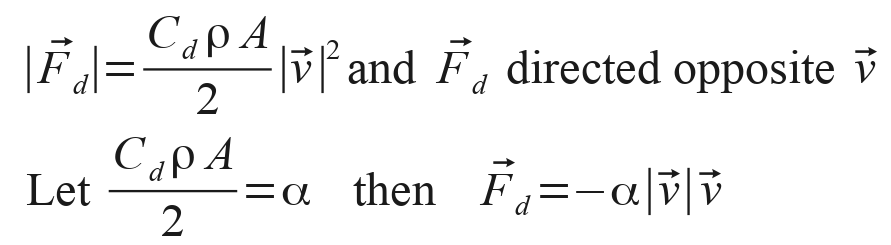
where Cd is the so-called "drag coefficient", μ is the fluid density, and A is the cross sectional area of the object. For the purposes of this interactive simulator we can bundle all the constants in this relation together as one coefficient α as shown. This expression above will generate an approximate air drag force with a magnitude dependent on the square of the projectile velocity and with a vector direction opposite to the instantaneous velocity.
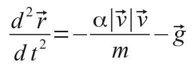
With the initial velocity vector v⃗ established by the launch, the projectile position vector r⃗ will be the solution of the second order differential equation
The vectors r⃗ , v⃗ , and g⃗ may be decomposed into two components in the x and y directions, giving a system of two scalar differential equations
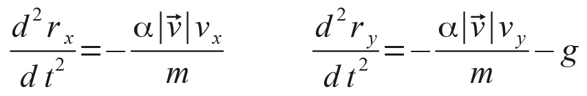
This system is now in a form that can be solved numerically to simulate the time dependence of the position and trace the projectile's trajectory.
The interative simulator at the top of this page will solve this time dependence and plot the trajectory determined by the parameters of initial launch speed, launch angle, and drag coefficient α input on the sliders. The projectile's position is plotted at each of the discrete time steps used in the numerical solution. The default very small value for α = 10-6 will give a solution very close to a simple parabolic path, but by adding in some significant drag, with α = 10-3 for example, you can see a distortion from the ideal parabolic path and a loss of range that must be compensated for by increased launch velocity.
Back to Computational Physics Playground page
Back to John Fattaruso's home page