The simple harmonic oscillator consisting of a single mass and a linear spring exhibits simple sinusoidal motion, but much more complex behavior can be seen by coupling multiple oscillators together by using common springs between the masses.
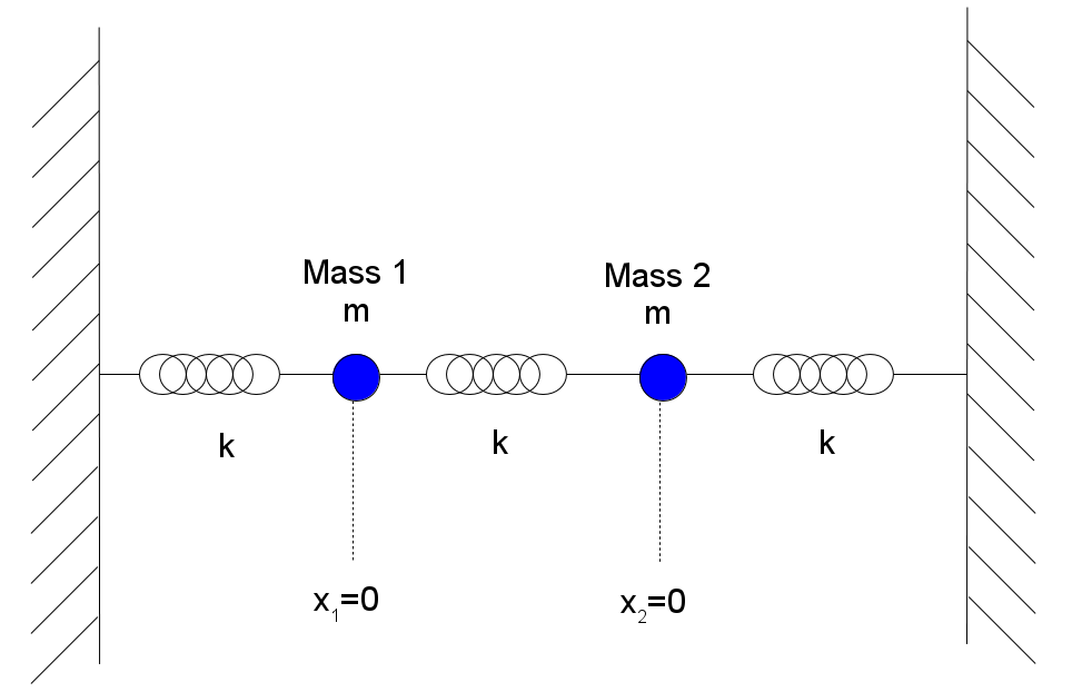
Consider the two-mass coupled oscillator shown here:
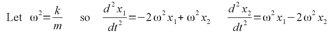
We'll assume that both masses are identical, as are the three spring constants. The displacement of each mass away from its equilibrium position is measured by the coordinates x1 and x2, respectively. The two simultaneous equations of motion that must be satisfied can be derived easily by either Newtonian or Lagrangian mechanics, and are:
Note that these are coupled equations, in that both motion equations have terms of both of the mass displacements. In order to seek out the so-called normal modes of oscillation, that is, the manner of motion where both masses are engaged in simple harmonic motion at the same frequency and time phase, but possibly different amplitudes, we first postulate that there will be solutions following the general form of
and then solve for the conditions that will allow this solution to be valid. Plugging in these assumed solution forms back into the system of equations of motion condenses down to the matrix relation
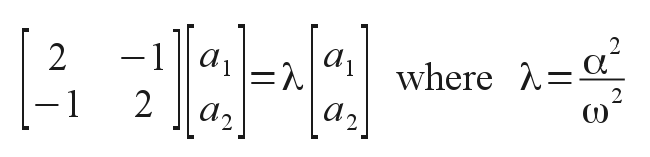
This is in the form of a classic eigenvalue problem from Linear Algebra. Solutions exist only at certain allowed eigenvalues of the parameter λ and for certain eigenvectors of the two corresponding oscillation amplitudes. For the coefficient matrix shown finding the eigenvalues is particularly easy, and gives
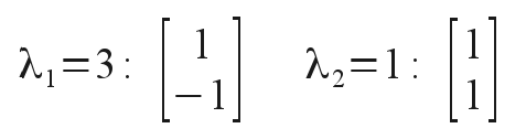
for the two allowed normal states. (Plug these eigenstates back into the original equations of motion and watch the coupling disappear!) Now a complete solution of motion of both masses may involve arbitrary linear combinations of these two independent normal modes. Translating into a more practical form of solution with sinusoidal and cosinusoidal (instead of complex exponential) terms, we have
The particular values of the ci coefficients are determined by the initial conditions applied to the oscillator. For instance, we may eliminate all the sin() terms simply by choosing an initial condition where the initial velocities of the masses are both zero. The general solution then reduces to
We can then excite one normal mode or the other by suitably choosing the initial mass displacements before releasing the oscillator for its natural motion. Choosing initial displacements that exactly match the eigenvectors will excite only the corresponding mode of oscillation, at its characteristic frequency. You can see the two normal modes in action with the application below by setting the initial displacements to either x1=1 and x2=-1, or to x1=1 and x2=1. Note the two different oscillation frequencies that ensue, corresponding to the different value of λ and therefore α. Other initial displacements give mixed mode oscillations, which are more complex, but ultimately can be resolved into some linear combination of the two normal modes.
The application below is also capable of simulating the more complicated motion of a three-mass coupled oscillator, pictured here:
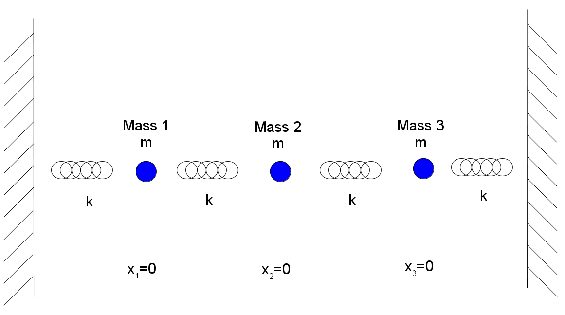
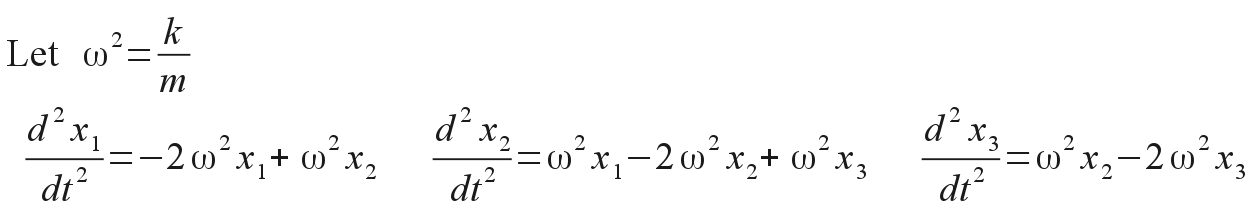
Derivation of the predicted motion proceeds as above, extending the equations to three masses. Again assume that all three masses are identical, as are the four spring constants. The displacements of each mass away from its equilibrium position become the coordinates x1, x2 and x3, respectively. The three simultaneous coupled equations of motion are then:
In order to seek out the normal modes of oscillation, we again postulate that there will be solutions following the general form of
and then plug in these assumed solution forms back into the system of equations of motion to solve for the conditions that will allow this solution to be valid. This condenses down to the matrix relation
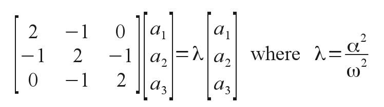
Now solutions exist only at three allowed eigenvalues of the parameter λ and for certain eigenvectors of the two corresponding oscillation amplitudes. For the coefficient matrix shown finding the eigenvalues is not as easy as in the two-mass case, but gives
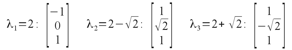
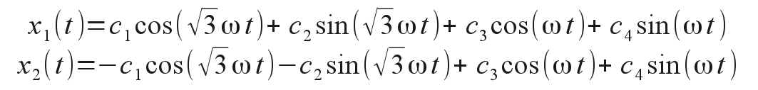
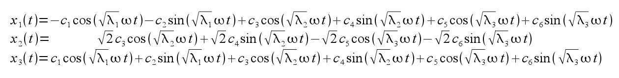
for the three allowed normal states. As before a complete solution of motion of all masses may involve arbitrary linear combinations of these three independent normal modes. Translating into a more practical form of solution with sinusoidal and cosinusoidal terms, we have
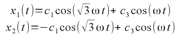
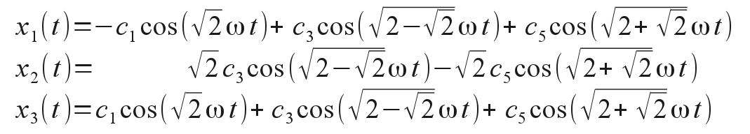
The particular values of the ci coefficients are determined by the initial conditions applied to the oscillator. For instance, we may eliminate all the sin() terms simply by choosing an initial condition where the initial velocities of the masses are all zero. The general solution then reduces to
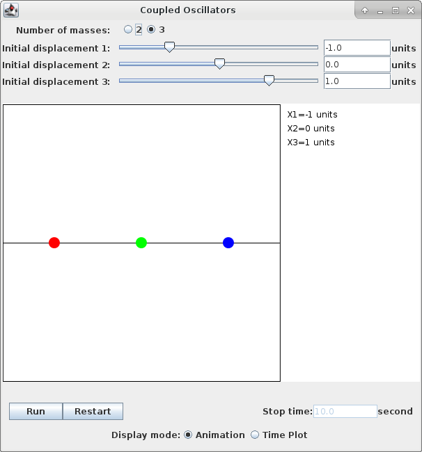
We can then excite one normal mode or the other by suitably choosing the initial mass displacements before releasing the oscillator for its natural motion. Choosing initial displacements that exactly match the eigenvectors will excite only the corresponding mode of oscillation, at its characteristic frequency. You can see the three normal modes in action with the application below by setting the initial displacements to either x1=-1, x2=0 and x3=1, or to x1=1, x2=1.414 and x3=1, or to x1=1, x2=-1.414 and x3=1. Note the three different oscillation frequencies that ensue, corresponding to the different value of λ and therefore α. The initial state of the application below is for a three-mass oscillator in the first of these three listed eigenstates. Other sets of initial displacements give mixed mode oscillations, which are more complex, but ultimately can be resolved into some linear combination of the three normal modes.
Run from a shell or command terminal in the download directory with:
java -jar CoupledOsc.jar
This coupled oscillator application works by directly solving the system of differential equations of motion with the Runge-Kutta algorithm, so you may experimentally verify all of the modal relationships above.
Back to Computational Physics Playground page
Back to John Fattaruso's home page