In the wonderful Deutsches Museum of Science and Technology in Munich, Germany, there is a splendid display of a real physical double pendulum that exhibits dramatically chaotic motion. You can watch a video clip I took on my visit. The pendulum is contained in a clear plastic frame, with the central shaft emerging. A visitor is able to start the chaotic motion by giving the shaft a good twist and imparting some angular momentum.
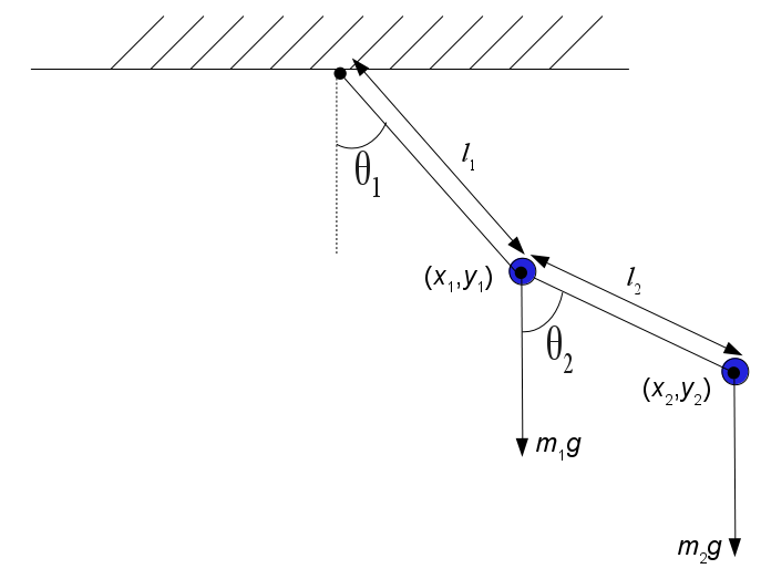
The geometry of a somewhat idealized double pendulum that is more readily analyzed is:
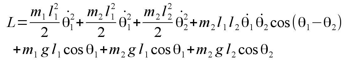
Rotating around the central free pivot there are now two distinct masses, m1 and m2, with the inner mass m1 located on a second freely rotating pivot. Instead of just one length, now the lengths of two segments of massless arm, l1 and l2, are adjustable parameters. Since the dynamic state of this physical system is now dependent on two variable angles, there will be two simultaneous differential equations required to completely characterize the motion. The differential equations of motion may best be derived by the Lagrangian method. The Lagrangian L is defined as L = T - V, where T is the sum of the kinetic energy of the two masses, and V is their total potential energy. For the system pictured above, this can be derived as
From this definition the Euler-Lagrange equation is applied twice with respect to the two angle variables θ1 and θ2 to derive the two simultaneous equations of motion:
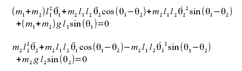
After some additional derivation, these may be put in a form that can be solved numerically to simulate the time dependence of the two angles. There are four initial conditions that must be specified, the two initial angles θ1 and θ2 and the two angular velocities dθ1/dt and dθ2/dt. Note that in the physical museum pendulum above, only dθ1/dt can be given a nonzero initial transient, and the angle θ2 is unreachable.
Due to the extra flexibility of the additional pivot, stable simple harmonic motion is not possible for this system, but both quasi-periodic and chaotic motion are readily observable. As in the physical museum pendulum, initially giving a large dθ1/dt and a small initial dθ2/dt will tend to lead to chaotic behavior. Assuming it is possible, as in the theoretical system in the figure above, giving both dθ1/dt and dθ2/dt similar initial values will tend to initiate stable quasi-static behavior.
As examples, the following are some simulated plots for two different sets of initial conditions. Since there are four state variables in this dynamical system, and four dimensional plotting is not possible to visualize, we cannot present a full state diagram. However, just looking at two of the state variables, namely the two angular velocities, a marked difference between quasi-periodic and chaotic modes is readily apparent. Consider first setting the initial conditions of both dθ1/dt and dθ2/dt to 10 radians/second. The following plot shows the regular pattern of quasi-static motion:
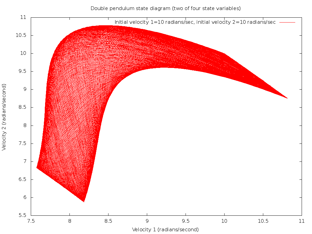
These initial conditions cause the motion of the double pendulum to be dominated by both masses rotating around and around the center pivot at a common angular velocity, with a little flexing or wobbling of the second pivot.
As in the case of the single pendulum, we can generate an audio track that corresponds to this motion by using the simulated angular velocities of the two masses as two audio signals, sampled at a much higher rate in time. In the case of the single pendulum this gave a monaural audio track, but since there are two angular velocities for the double pendulum, these can be arranged into a stereo track:
Note that with the quasi-period motion the corresponding sound track is dominated by discrete tones. Another way to induce quasi-periodic motion is to only spin the inner angle initially, and at a low velocity, so the pendulum will just wobble back and forth. This stereo audio track corresponds to the initial conditions of dθ1/dt=5 radians/second and dθ2/dt=0:
In contrast, setting initial values of dθ1/dt=10 radians/second but dθ2/dt=0 demonstrates a chaotic plot of completely different character:
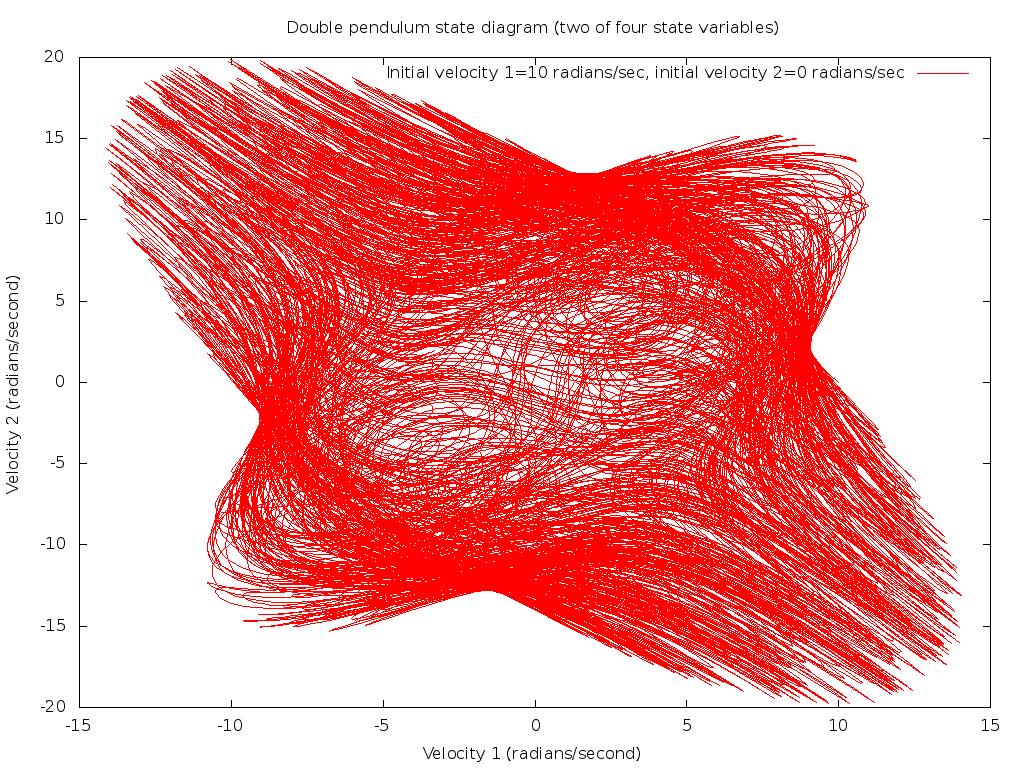
As before we can digitally compose a stereo audio track by sampling the two angular velocities, and for this chaotic case results in a sound pattern of a completely atonal character:
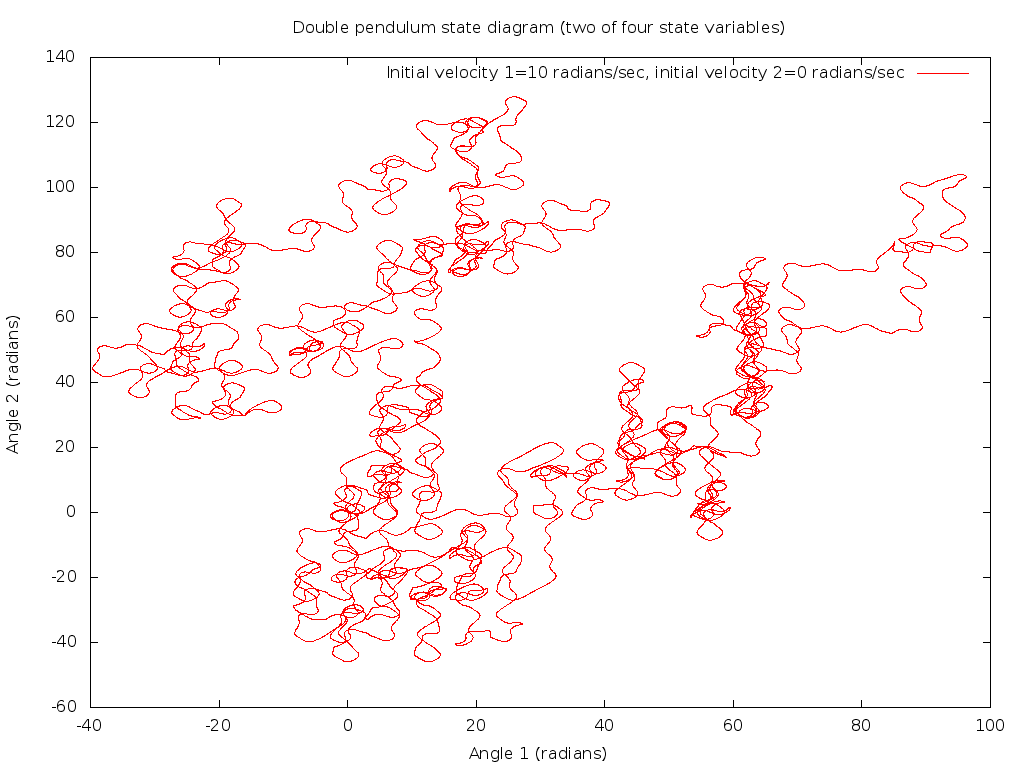
It is also interesting to see two different state variables plotted against each other, the two displacement angles θ1 and θ2 in chaotic mode:
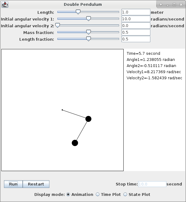
Run from a shell or command terminal in the download directory with:
java -jar DoublePendulum.jar
Note that two parameters you are able to adjust in this application are called the "mass fraction" and "length fraction". The mass fraction α, a value between 0 and 1, is defined to be m2 / (m1 + m2), or in other words, the fraction of the total mass that is associated with the outer weight. Similarly the length fraction β, also a value between 0 and 1, is defined to be l2 / (l1 + l2), or the fraction of the total pendulum length between the inner and outer masses. The values of these two parameters are a large determining factor whether the pendulum motion is quasi-periodic or chaotic. A small or large length fraction value, placing the inner weight toward either inner or outer end, tends to stabilize the motion into quasi-periodic mode, whereas length fractions around 0.5 tend to lead to chaotic motion.
You may adjust the various parameters controlling the simulations by either moving the sliders or by typing in a numerical value and hitting the Enter key.
To study the range of values of the two parameters α and β that lead to quasi-periodic or chaotic behavior, it is convenient to have a numerical measure that indicates the class of motion that may be plotted with respect to the parameter values. One easily computed metric is the Weiner entropy, or spectral flatness metric. If we take the Fourier transform of one of the mechanical measures of the double pendulum, for example, the angular velocity of the first member dθ1/dt, the spectrum will consist of only a series of spikes for quasi-periodic motion, but will spread out into a noisy base under chaotic conditions. The entropy of the spectrum will be low, close to 0, when its energy is concentrated in a few spikes, but much higher, close to 1, for noisier spectra.
As examples of how this measure predicts the regions of chaotic and quasi-periodic pendulum behavior, consider the first plot:
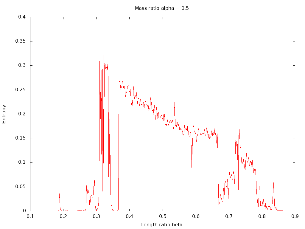
This shows the spectral entropy of the angular velocity of θ1 plotted versus β, with α set to the equal masses value of 0.5. Note that chaotic motion, associated with high entropy values, is only present for length ratios in the vicinity 0.5, the case of equal arm lengths. In contrast, the second entropy plot:
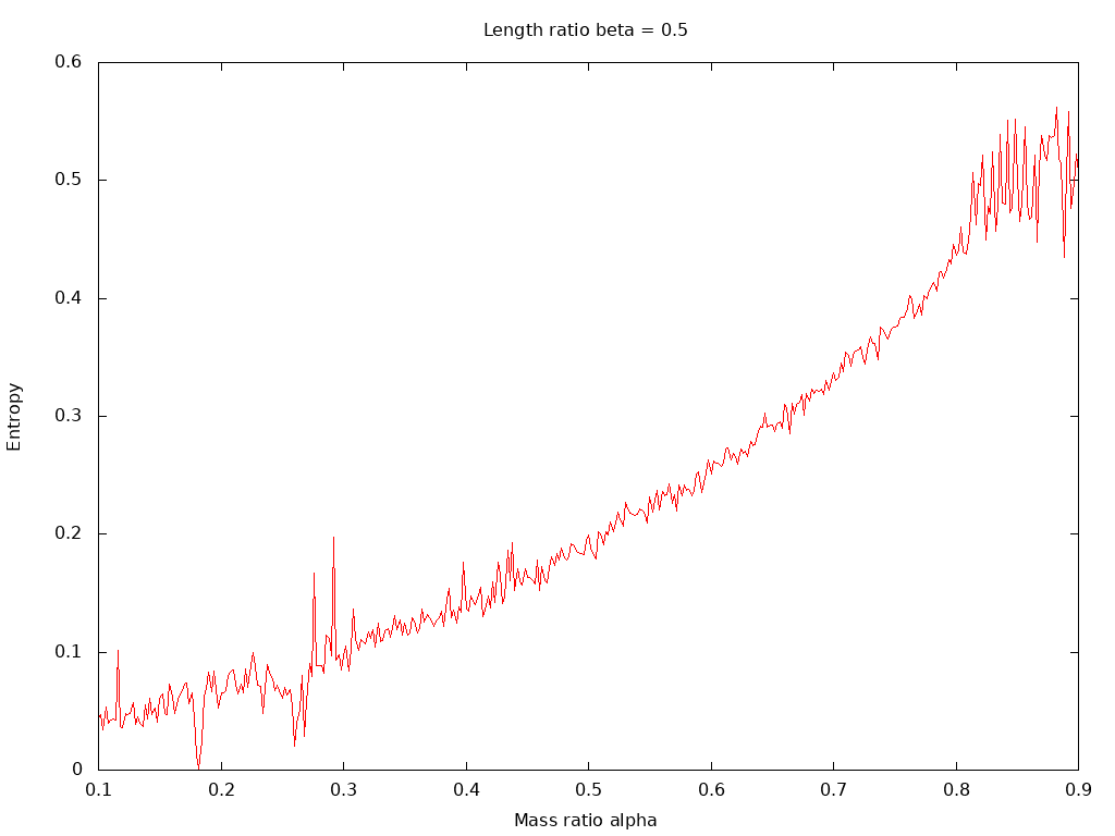
plotting entropy versus α with β set to 0.5 for equal lengths, shows that the presence of chaotic motion over a much wider range of the mass ratio.
The final plot is a three dimensional projection of the entropy as both α and β are varied over their practical ranges of 0.1 to 0.9:
Back to Computational Physics Playground page
Back to John Fattaruso's home page