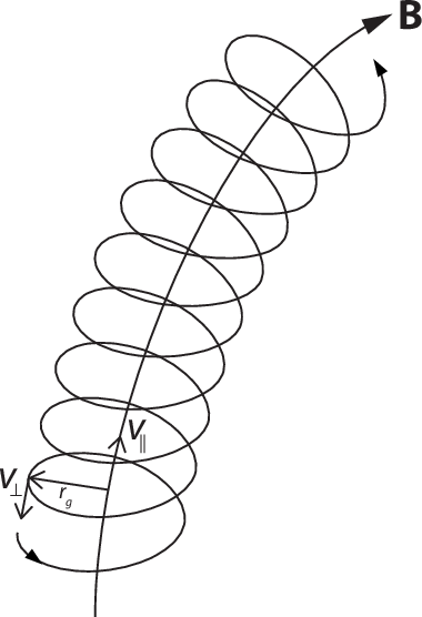
It is well known that a moving charged particle immersed in a uniform magnetic field traces out a helical path around the B field lines. The force on the particle will be F⃗ = qv⃗ × B⃗, and the motion may be seen by decomposing the velocity into components that are parallel and perpendicular to the B⃗ field direction. The parallel component of the particle's velocity will be unchanged, and the perpendicular component to the field will form the tangential velocity around a circle, with the magnetic force forming the centripital force. The superposition of these two velocities gives a helical path:
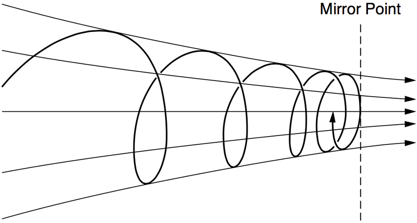
When the field intensity increases locally and the field lines reach a critical level of convergence, a thorough mathematical analysis shows that there are constraints on the velocity, and under some conditions the parallel velocity component must suddenly reverse. This results in an apparent "reflection":
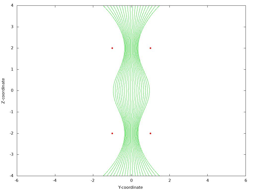
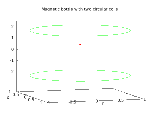
Numerically simulating this phenomenon is fairly straightforward, although a little involved due to the need to track three dimensions. The nonuniform field is generated by two parallel circular coils carrying a constant current. The separation of the coils is increased relative to the classical Helmholtz arrangement that gives a uniform field in the center. By spreading out the coils, the field goes through a minimum at the center, and then the field lines converge toward the center of both the upper and lower coils as the field increases. With this symmetrical arrangment, any charged particles in the center with a vertical component of their velocity will experience reflections near both the upper and lower coils, and thus be confined within this "magnetic bottle". The field lines between the coils in a plane through the coil centers with this increased separation is shown here:
The outer level computation is a simulation of the vector equation of motion a⃗ = (q/m) v⃗ × B⃗ with a Runge-Kutta solution of the second order differential equation in three dimensions. An automatically variable time step must be used to carefully step through the reflection events to avoid algorithm instability, as the velocity momentarily goes through a peak. Then within each time point iteration of the differential equation solution, the local field intensity must be computed with a numerical spatial integration of the Biot-Savart law. This is realized with a simple Simpson's rule integration, although keeping track of the three dimensions of the B field. In the simulations below, each circular current path is broken into 72 samples around its contour. A charged partical is given an initial velocity in the center of the arrangement, and as the simulation proceeds, the helical motion in the center and the reflection phenomenon near the top and bottom are clearly evident:
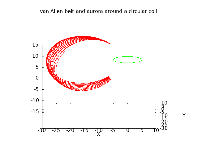
A similar reflection takes place near the magnetic poles of the earth. As the field lines converge near the poles, charged particles from the solar wind get trapped and cycle back and forth from north to south. The plot below is the result of a similar simulation, but now with a single circular coil, shown in green, carrying a current that forms a magnetic dipole similar to the earth's magnetic field. A charged particle is introduced with velocity above the earth, and its simulated path is shown in red with a series of reflections near the north and south magnetic poles. The helical path of the reflections can also cause a rotational drift around the earth. This forms the charged layer known as the Van Allen belt:
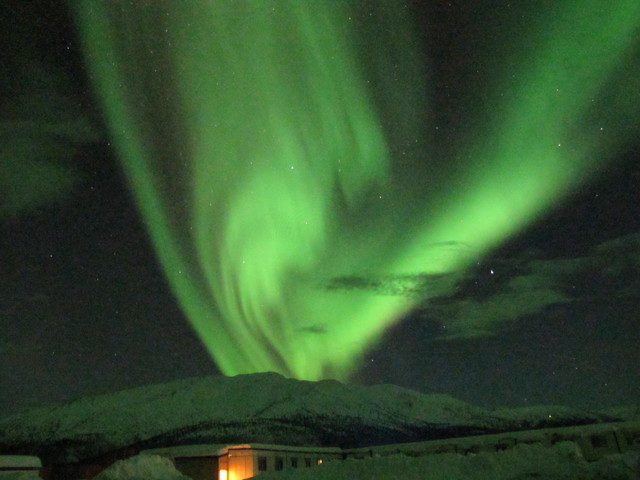
Some particles will not satisfy the reflection constraints and will be sent all the way into the atmosphere around the so-called "aurora oval". These electrons have sufficient kinetic energy to ionize gasses in the atmosphere and induce flourescence. Below is a photo of the Aurora Borealis taken north of the Arctic Circle in January of 2016:
Back to Computational Physics Playground page
Back to John Fattaruso's home page