The single pendulum is a deceptively simple physical system that is capable of rich dynamic behavior. By adding damping effects and torsional forcing, the physical behavior can exhibit periodic, quasi-periodic, or chaotic motion.
The most basic form of the single pendulum is
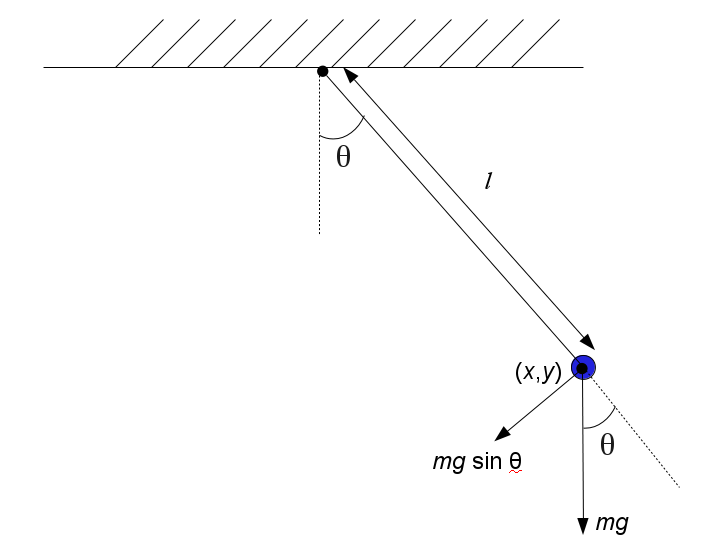
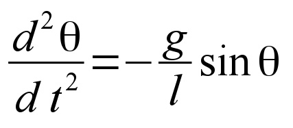
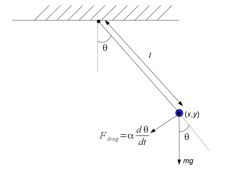
The angle θ measures the displacement of the (massless) rigid pivot arm with respect to vertical. A mass at the end of the arm, at a distance l from the pivot point, is subject to a downward vertical gravitational force of mg. The component of this force that generates a rotational torque is mg sin(θ). Analysis of the angular acceleration induced by this torque gives the well known nonlinear differential equation:
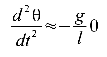
In elementary Physics textbooks this is usually solved by applying the simplifying small angle approximation, that is, if θ is small, then sin(θ)≈θ. In this limiting case the differential equation governing the motion reduces to the linear equation
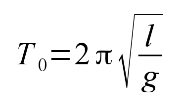
It is well known that the solution of this differential equation, given an initial nonzero displacement angle, is simple harmonic motion, and the function of angular displacement θ will be in the form of sines and cosines of time, with a period given by
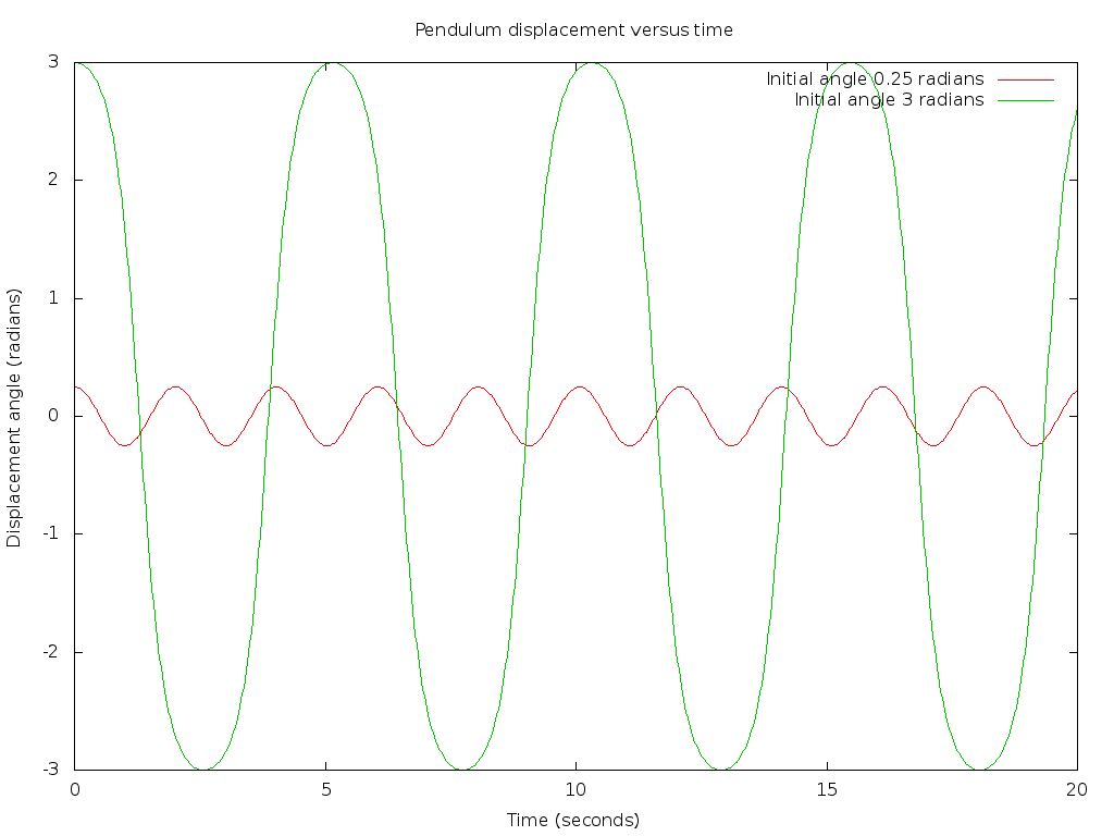
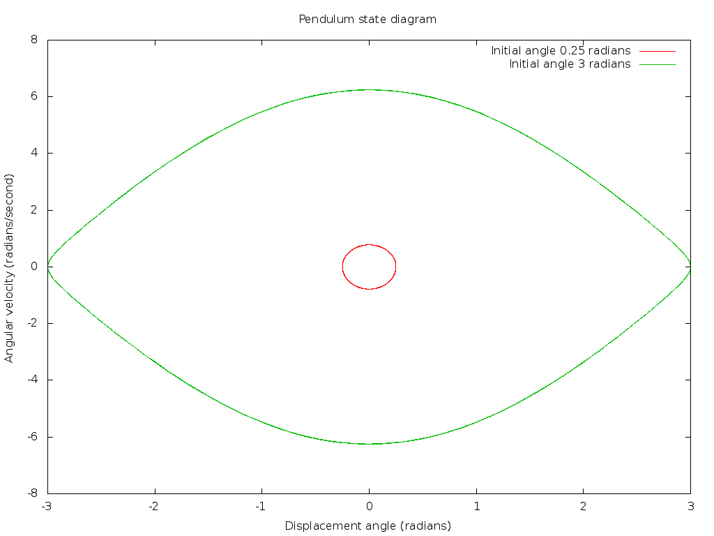
Now the more general case is that an initial angle is established which is not necessarily small, and the above small angle approximation is not valid. In that case the differential equation remains nonlinear, and unfortunately does not admit an analytical solution. However, it may be readily solved by numerical means. As an example, consider the following plot. This shows the result of two simulations of a 1 meter long pendulum, one with an initial displacement of 0.25 radians, and another after setting an initial displacement of 3 radians. Note the cosinusoidal motion with a period of about 2 seconds in the small angle case, but that the solution for large angles is markedly distorted with an extended period. This is due to the pendulum spending a relatively long time over the peaks of displacement when the angle is large. (What simple physical reasoning can explain this period lengthening?)
Now imagine speeding up the motion of the pendulum by a factor of about 1000 and converting the resulting oscillation to an audio signal. This audio file is the sound that corresponds to a pendulum with an initial angle of only 0.1 radian:
Note that its timbre is a pure, single frequency tone, as the differential equation solution for this small angle is almost purely sinusoidal. In contrast, the audio corresponding to an initial angle of 3 radians can be heard here: Note that not only is the frequency considerably lower, but the timbre is less pure, indicating a distorted wave with the presence of overtones.Now consider the addition of two other torques on the rotation of the pivot arm. The first is a damping force, perhaps by air resistance or friction in the pivot, that is assumed to be proportional to the angular velocity dθ/dt. This damping torque is illustrated in the following diagram:
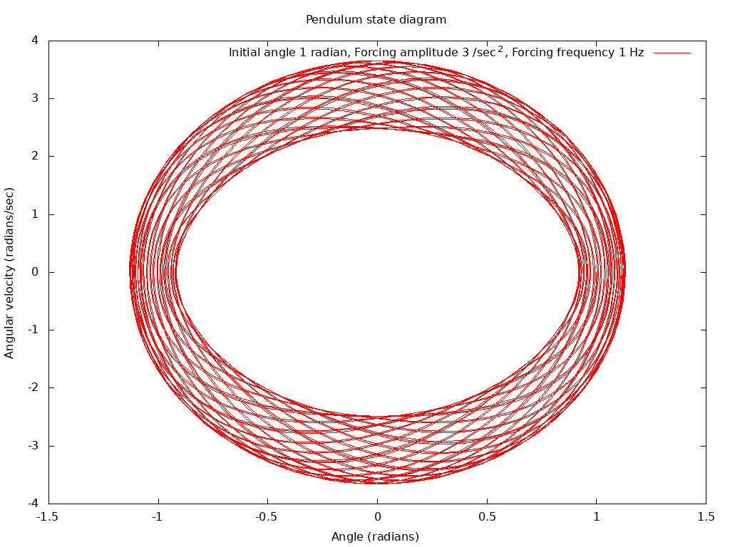
The second additional torque is sinusoidal forcing, for example applied by an electric motor connected to the pivot shaft. The governing differential equation then becomes:
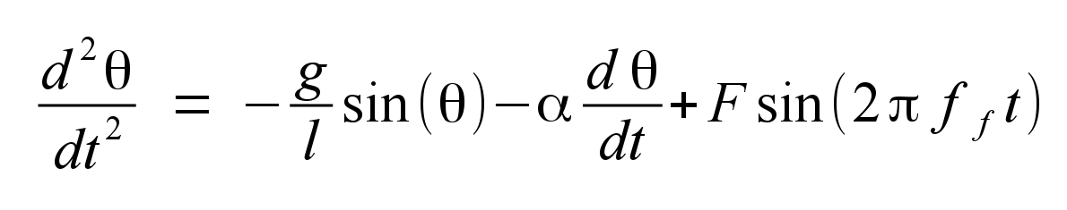
where α is the damping coefficient, and the forcing amplitude and frequency are specified by the constants F and ff. Note that the forcing torque is a sinusoidal function with, in general, a frequency ff unrelated to the natural period of the pendulum oscillations.
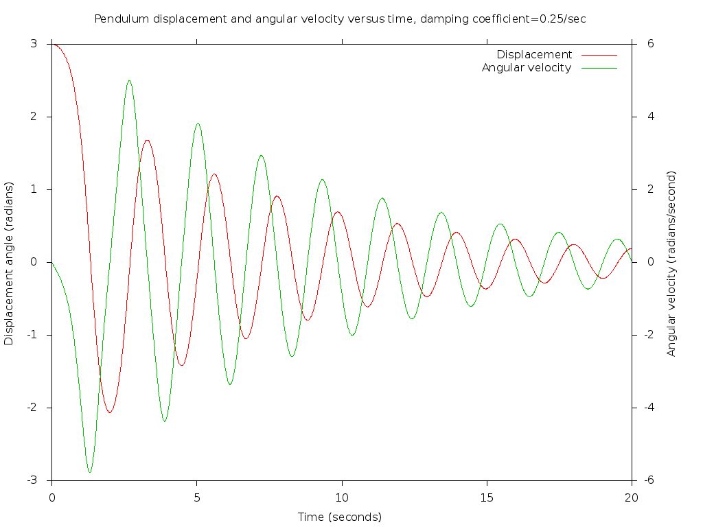
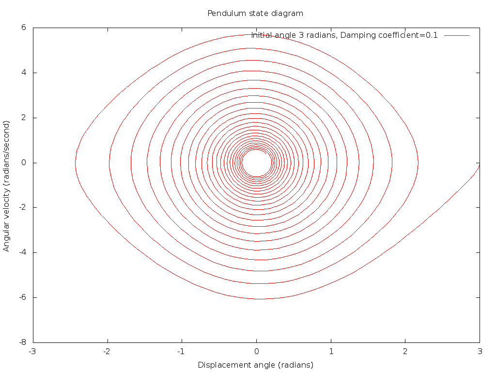
Introducing some damping will cause the pendulum oscillations to damp out exponentially with time, as illustrated in this plot for a damping coefficient of 0.25/sec. Note that in this plot we can see both the angular displacement and the angular velocity as a function of time plotted together. The initial angle is 3 radians, and the initial velocity can be seen to be small. Where the initial velocity is small, the period is extended, and then the period shortens as the amplitude dampens out, as the small angle approximation becomes more valid and the solution to the linearized differential equation applies.
More complex behavior of the pendulum is best pictured by a different sort of plot, one where the displacement angle is plotted against the angular velocity. The instantaneous state of this dynamic system can be described by the values of these two "state variables", and will determine the evolution of the solution for all future time. As time evolves, the intersection point on these two axes rotates around in a path. If there is no damping, conservation of energy constrains the motion around a closed path, and one that is elliptical in the limit of small angles. With some damping, the figure will collapse to the origin and become more elliptical as energy is dissipated over time:
For most selections of the two frequencies, the behavior of the pendulum system is what is called "quasi-periodic". That is, the natural oscillation frequency and the forcing frequency are mixed and locked by the nonlinearity of the differential equation in a complex way that produces a periodic motion, but with an overall period that is some rational fraction multiplied by the forcing frequency.
This audio file is the sound that corresponds to a forced pendulum in quasi-periodic motion:
Note that there are different distinct audio tones present, as a result of the nonlinear interaction of the two physical frequencies.However, for certain ranges of forcing frequency, the behavior of the pendulum becomes dramatically chaotic. The state plot appears to spread out in wild looping behavior:
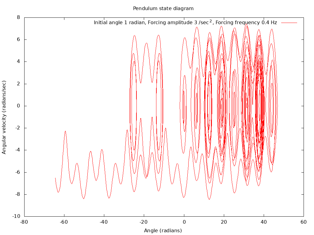
What is the physical significance to displacement angles increasing to the tens of radians on this plot? Another hallmark of chaotic behavior is that this plot would describe a radically different trajectory through the state space if the initial condition or forcing parameters were to be altered by tiny numerical amounts.
The sampled audio file generated with these chaotic parameters sounds completely different, completely aperiodic:
Run from a shell or command terminal in the download directory with:
java -jar SinglePendulum.jar
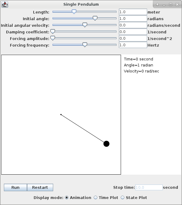
With this introduction to the physical principles of the single pendulum, the following application will let you play with the various parameters and observe the numerical simulation of the equations of motion. Note that the display mode can be switched from an animated physical view to the two plot modes by use of the check buttons at the bottom.
You may adjust the various parameters controlling the simulations by either moving the sliders or by typing in a numerical value and hitting the Enter key.
Back to Computational Physics Playground page
Back to John Fattaruso's home page