Focal Length and Image Size: Here's notes about the sections.
- Distance from lens to light: We'll measure this for each team. You'll have to help me with this;
we'll use the measuring tape and it takes two to do it.
- Record lens data: The lens name will have to be the data on each lens mount. The diameters are
all the same; measure one yourself and record it. The focal length here is interpreted as the image
distance. Image size is the length of the image of the fluorescent tube.
- Plot of image size vs lens diameter. Since all lenses are the same diameter this plot should
be a straight line along constant diameter.
- Plot of image size vs focal length. This should be a straight line of image size increaasing
with focal length.
- Relation between image size and lens diameter. This is a straight line parallel to the
diameter axis. No useful relation exists; given a lens diameter you cannot predict the image size.
- Relation between image size and focal length. There is a direct relation between the two;
image size increases linearly with focal length. Given a focal length you can predict image size.
- What happened to the image with half the lens covered? The only change is that image is dimmed;
it is not cut in half.
- Compare part 3 and part 4 focal length results. The focal lengths for part 3 and part 4 should
be a bit different, part 4 being about 10% longer. Reason: part 3 uses both object and image distances
to find focal length. In part 4 we take image distance to be focal length, ignoring the object distance.
This yields a focal length that is longer than actual. Object distance can be ignored only if it is
large enough to make the 1/objectdistance term approach zero. The Moon is a good example.
- Recalculate focal length from part 4 data. This should produce part 4 results that are close to part 3.
The reason for the improvement is including the 1/objectdistance term; if the object is not far
enough away to make the term approach zero you need it.
Lab 4 - The Lunar Surface
This one involves studying lunar surface photographs taken by Luner Orbiter spacecraft around 1965.
The idea is to find out something about the Moon's surface and its history. That's one of purposes
that these photos were uswed for in the late 1960s. The primary purpose was landing site selection
for Project Apollo.
Analysis and Measurements
- Analysis
- Classification Scheme: This involves studying the photos and identifying classes of features
that might reveal something about the Moon's surface properties. Something that is just a "crater" doesn't
help much as the surface is covered in craters. See if they found interesting features that are NOT common.
THere are some ripples, bright rays. mountains, dark flat areas, dark/light boundaries, and more.
They will assign a name to each type of feature; look for reasonable names, not "hamburgers" or "piles."
- Find examples (not graded): Here they give the coordinates of the features as found on the
copies of the photos which have coordinates on both axes. Check to see that you find the named feature
where it is said to be. Also - it is not necessary that they fill all of the spaces; leaving 3 or fewer
blank is OK
- Determine relative age: There are places where you see two different features interacting;
in these cases you can often see which one was there first. You can't get the time between the formations
but you can determine the order. Example: two craters, one located in the outer wall of a larger one.
Obviously the impact which damaged the shape of another feature is the younger.
- Older areas: The dark, flat areas are mare (mah-ray) areas. The ancient observers thought they
were oceans or seas, as that's what they sort of look like. The more rugged and mountainous areas are
the lunar highlands. The highlands are older, although you can't tell by how much. Mare material, which
was once molten like lava, flowed up against higher terrain of the highlands. This is evidence that
the highlands were there first. Also - if you look at crater density - you will see that the mare areas
have far fewer craters per unit area than the highlands. This implies that the mare were exposed to
impacts for much less time than the highlands and are younger.
- Height of mountain: Finding the height of a mountain is conceptually easy. Looking down from
orbit we can see the mountain's shadow and measure its length from the distance scale. That horizontal
feature along with the height of the mountain make a right triangle. All you need is angle at which
the shadow intersects the ground, which is Sun elevation. That we don't have. Look for a description of
the method plus a note that we actually can't do it because we lack Sun elevation data.
- Hills and holes: The trick is to distinguish be a hole (crater) and a hill. This is easy.
The student need only look at the shadow they see. A hill has its shadow opposite the Sun and a hole
has a shadow inside it on the side toward the Sun. Look for understanding of this.
- Size of smallest crater: This requires looking for a VERY small crater. They should be able
to find one less than 1mm diameter. They will then use the distance scale on the copy of the photo
to estimate that crater's size. It is normally less than 1km.
- Conclusions:
Lab 5 - The Earth's Orbital Velocity
Analysis and Measurements
- Record Measurements in millimeters: Spectrum a is redshifted; spectrum b is blueshifted.
Look to see if all the measurements (7) are similar as expected. Spectrum a shifts are not the same
as spectrum b shifts. Shifts in spectrum a are close to 1.5mm; in spectrum b they are about 2.5mm.
- Record Scale of the Spectrum: The distance between lines 1 and 7 is approximately 280mm.
The lines wavelengths are 47 Angstroms different; this yields a scale factor of approximately 0.17.
The calculation is 47/280. After this it's all calculation.
- Redshifts and Blueshifts:This is calculated by multiplying the shift distance (mm) by
the scale factor (Angstroms/mm). These should be under 0.5 Angstrom. The values in each column should
similar - look for any that stand out as different.
- Redshift and Blueshift Velocities: They convert shifts in wavelength to velocity using the
Doppler shift formula as shown in the lab text. These will be double-digit km/sec.
- Calculated Value for Vo: The formula for this is in the lab text. Vo
is in the area of 30 km/sec.
- Calculated Value for Vs: The formula for this is in the lab text. Vs
is in the area of -5 km/sec. The minus value means that the star is aproaching the Sun.
- Earth-Sun Distance:This is done by calculating the number of seconds in a year then multiplying
that by the determined valocity, giving the circumference of Earth's orbit. Dividing this by 2pi gives
orbit radius, which is the Astronomical Unit.
- Compare to Accepted Values:This is not graded. It just allows evaluation of the results. You can
use it to evaluate how close they got. A large error calls for a bit of investigation. Calculationj error
is a likley culprit.
- What Kind of Errors...: For the first time I'm going to ask that the spectrum sheet be turned in;
this will let you inspect them for some mechanical errors. Here are some possible error factors:
- Error drawing reference lines. These lines must connect the top and bottom lines of each pair
center to center. If the line is off to right or left it will cause error.
- Fuzzy edges of absorption lines. The edges of the absorption lines in this magnified copy of a half-tone
image are not sharp. There is some uncertainty about where the line edge is.
- Zero-setting error in measuring. This is the usual problem of not getting the ruler's zero set right.
- Not measuring correctly - from reference line to center of absorption line.
Lab 6 - The Orbit of Mars
the division
This exercise has two parts: drawing and measuring ellipses and then using data from Tycho Brahe to plot
the orbit of Mars. The ellipse part is for background for discovering the ellipse that is Mars' orbit.
Analysis and Measurements
- Drawing Ellipses: The students will draw 3 ellipses using 2 pins and a loop of string.
This is a correct means of drawing an ellipse. They record 3 values for each ellipse:
- F1 to F2: This is the distance between the foci (the pins).
- Major Axis: Total length of the major axis measured along the central line the pins are on.
- Eccentricity: Divide F1-F2 by the major axis length. This WILL be less than 1. A result
greater that 1 indicates the division was upside-down.
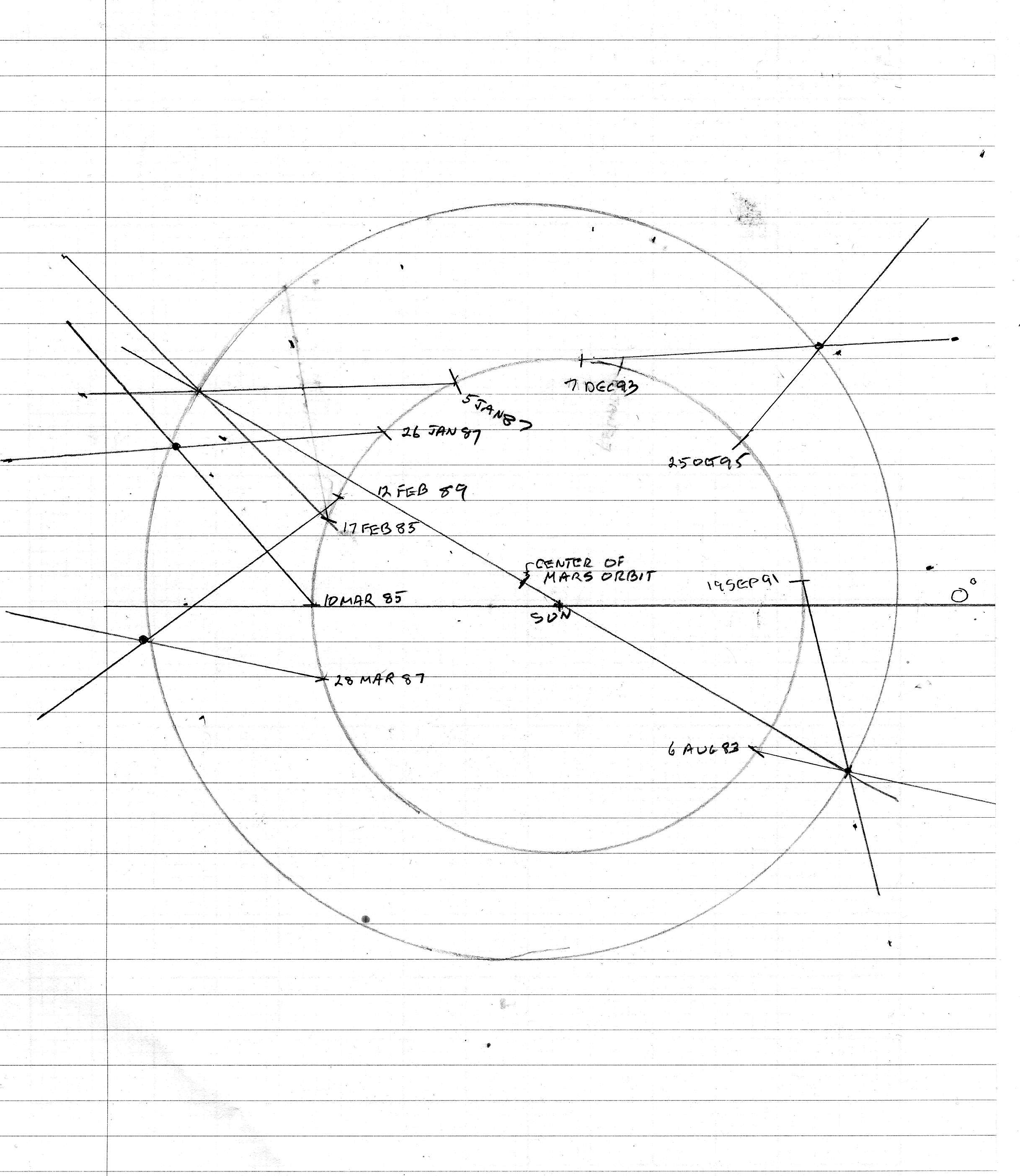
- The Orbit of Mars: This is a somewhat complex exercise in plotting data. We need to
circulate while they do it, checking their work to prevent major goofs; this is preferable
to having to correct a large error later. There are 5 data pairs to plot. They will use a page
having a Sun point near the center of the sheet and on one of the blue page rulings. They
need a zero degrees line from the center (Sun point) to the right edge of the paper. Next, they
draw a 5 cm diameter circle for Earth's orbit. There are 5 pairs of data points in the text; each
pair of values defines one configuration of Earth and Mars. Heliocentric longitudes of Earth
are plotted with the Sun point as the center and the Earth mark made on the 5 cm circle.
I'll instruct them not to draw the line here, only to make a mark at the outer edge of the protractor.
They'll have to use a ruler to move that position to Earth's orbit. The geocentric longitude
of Mars is plotted from the matching Earth point on the 5 cm circle. This time they do draw
the line outward from the Mars point. For each pair of Earth/Mars points these two sight lines
should intersect outside of Earth's orbit in a reasonable position (I'll show you).
The first two pairs of positions in the data set define the major axis of Mars' orbit. They will
draw a line between those two points to show the major axis (be sure they do this!). Quick check:
the major should pass right through the Sun point (center), A major miss means one or both of
those first two Earth/Mars points is not plotted correctly. The usual error is not getting
a longitude angle right; some are in the 4th quadrant and they goof this.
I have scanned the plot I made Monday that you saw. Two plot are not there; they would be on the
left side., Check the student's of these to see that the points (intersections) lie on the orbit
circle or very close to it. Click here for the scanned plot.
- Record measured values
- Relationship of Earth and Mars
- Error Analysis:
- Conclusions:
Lab 7 - Measuring the Solar Constant
After you see how the measurements are done it will make sense. The idea is to use a glass jar
with black tape around half its inside to collect sunlight and heat water. One calorie of energy
heats one milliliter (1 cc) by one degree C. Make notes for yourself about sky/cloud conditions;
poor transparency will affect the measurements and we won't know about conditions till we see them.
After the first measurement each team will pour the contents
of their jar into a large graduated beaker to find water volume. Any of us can do this.
Analysis and Measurements
- Analysis: This section is the whole exercise.
- We make four 15 minute measurements: two with the jar in the Sun and two with the jar in the shade.
Each measurement is supposed to be exactly 15 minutes long. Check start and end times. Check to
be sure the temperature rise in Sun is significantly larger than in shade.
- Look at the final result - It should be in the area of 2 cal/min/cm2.
- If the result is far off check the calculations (the procedure gives it).
- Error Analysis: This measurement usually shows some error.
- Clouds are the obvious problem, resulting in a result that is low.
- Insufficient water in jar. If part of the tape is above water during the measurement the solar
energy collected will be low. We should inspect for this during measurements.
- Not exposing the jar for exactly 15 minutes can cause variation.
- Significant mispositioning of the jar can cause error. It needs to be exactly facing the Sun and
perpendicular to the incoming sunlight.
- Putting the jar on a concrete surface. If we are watchful during the measurements we can prevent this.
- Someone standing nearby casting their shadow on the jar is obvious. We need to be watchful for it.
Lab 8 - Measuring istance by Parallax
This one involves measuring the distances to three buildings on the campus: Simmons, Caruth II
and Fincher. The photograph availablw with the data sheets shows them as well as the ONLY
downtown building that can be used as a refefence. A very simple cross-staff measuring device
is used. It works very well for its simplicity. For your reference, the distances to the
buildings are (approximately):
- Simmons: 500 ft
- Caruth; 1160 ft
- Fincher: 1400 ft
These were measured on a Google maps aerial photo. That is usually good.
Analysis and Measurements
- Analysis: There are data areas for three target buildings; data to be taken are the
same for all three.
- Object name: This will be Simmons, Caruth or Fincher.
- Baseline length: This starts with 1000 ft. (53 ft for Caruth). Corrections for actual
measuring position are added for each end so actual baseline is known. Caruth is done
with a shorter baseline because of obstrucion by Simmons.
- Measurements: We take three measurements at each end fo reduce the effect of random error.
Meaurement quality can be assessed by looking at the range in the measurements. It is possible
to measure the angles with distance down the meter stick scattering within about 1 cm.
This can be achieved with care. A range of 3 cm or more is sloppy.
- Mean: The simple arithmetic mean (average) of the three measurements.
- Angles from ends of baseline: The equation at the bottom of text page 8-4 is used.
Check to see that the calculations are correct.
- Parallax Angle: Here a critical choice must be made. The actual parallax angle is computed
according to figures 5/6 or 7/8 depending on what is observed. If the target crosses from
one side of the reference point from one of the baseline to the other, use figures 5/6 (only
Fincher does this). Otherwise use figures 7/8 (Simmons and Caruth). One of the most common
mistakes is to use the wrong equation (figure) to compute this. Check for this.
- Distance: Use the last equation on page 8-8. With the baseline measure in feet, the result
will be feet. Note that "A" represents half the baseline length.
- Error Analysis: The only opportunity for measurement error is the actual angle measurements.
The aperture is out of focus in the eye when looking at the building - small uncertainty here.
It is not easy to hold the meter stick steady while measuring. Lining up the aperture edges
prescisely with the target and reference is tricky.
- Conclusions:
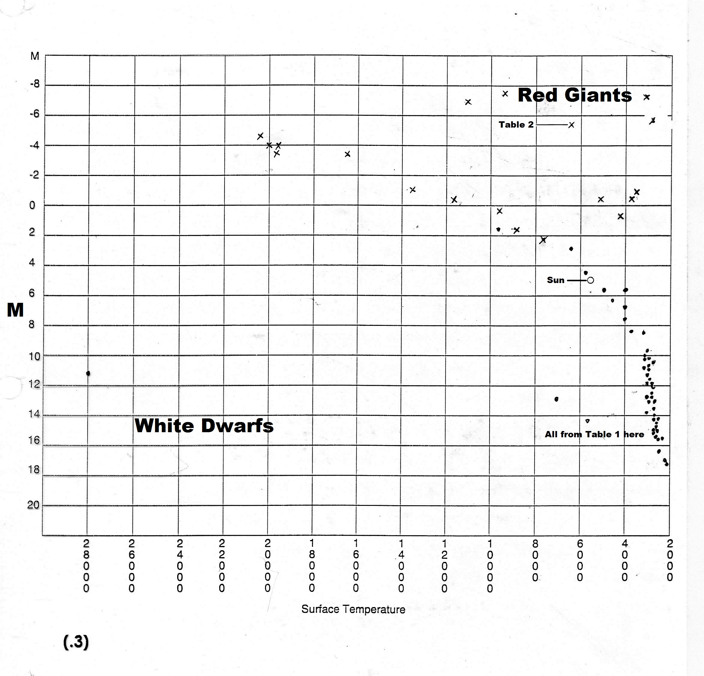
Lab 9 - The HR Diagram
The instructions for plotting the data are clear. We should circulate and check to be sure they are
actually following the instructions. For assessing the plots, I have transparencies (prepared by
Prof. Scalise) that you can use to compare their work to really accurate plotting. There's one of
these for each of you. Return them when done - we'll need them again. I have scanned one of these
plots for you. Here's the image; I added a few notes.
The equation they will use for magnitude calculations is m-M=5log(d/10). "m" is the apparent
magnitude (brightness) of the star on the sky, "M" is what the apparent magnitude would be if the
star were exactly 10 parsecs away, and "d" is the star's distance in parsecs. Magnitude numbers
are not intuitive: a larger number means a fainter star. The brightest star (Sirius) is mag -1.5.
The text of Lab 9 has this solved for each variable, plus more background.
Analysis and Measurements
- Most Numerous: The most numerous stars on the plot will be at the lower right.
These are the cool, red dwarfs (type M)
- More/Less Luminous: In Table 1 only three stars are more luminous than the Sun (M < 4.85).
- Diameter: The larger star will be 4 times more luminous. Surface area (4 pi r2)
of the larger one is 4 times that of the smaller.
- Luminosity Difference: Deneb is most luminous (M= -7.5). LP731-58 is least Luminous (M=17.3).
The difference is 24.8 magnitudes. This is approximately 8,300,000,000 times.
- Temperature/Luminosity: One of the stars should be in the Main Sequence band and the other
one some distance directly above it. The reason for different luminosities at the same temperature
is surface area; the brighter star is much larger.
- Sun Visibility: The apparent magnitude (m) will be 14.6. No chance of naked eye visibility.
Naked eye visibility means magnitude 6 or brighter (smaller number).
- Deneb: This distance is approximately 3800 parsecs.
- Sun Naked-Eye Distance: This distance is about 17 parsecs.
Lab 10 - The Crab Nebula
There's a lot of calculation in this one, so keep a lookout for calculation goofs. There's also
a lot of measurement. They will use the small rulers and try for 1/2 mm precision. We need to look at
some of the knots they have chosen and be sure they identify the exact same feature on both. Make sure
they understand this.
- Compute Scale Factors: The students will measure (in mm) the distance between the two stars
marked by white arrows. These stars are 576 arcseconds apart on the sky. Dividing 576 by the measured
distance will give the scale factor for that plate. This must be done for both plates as they are
slightly different. The factors will be somewhere around 2.
- Record Distances: The students must identify 12 "knots" (maybe globs) around the outer
edge of the nebula. They must positively identify each knot in both plates. We need to circulate
and help them get this right. They will have to measure the distance from the neutron star (tiny black dot)
to the same feature on the knot in both plates. Sanity check 1: the nebula is really expanding, so the
distance in the 1976 plate must be larger than the 1942 distance. Sanity check 2: The 1976-1942
differences should be similar for all 12. If one difference is significantly different from the others
it should be checked. Be sure the students measured exactly the same feature of the knot on
both plates.
- Compute Angular Distances: Simply multiply the mm distance by the appropriate scale factor
to get arcseconds on the sky.
- Compute Angular Velocities: Divide the 1976-1942 difference by 34 (years) to get arcseconds
per year as the expansion rate.
- Compute Expansion Time: For each knot, divide the 1972 angular distance by the expansion rate
to estimate how long it took for the nebula to expand that far. The average of these will be the estimated
time from the explosion to 1976. The perfect result: 1976-1054=922 years.
- Estimated Year of Explosion:Now subtract the estimated time (years) from 1976 to estimate the
year the explosion was seen; it was observed in 1054.
- Discrepancy: Error in measuring distnces is the usual culprit here; look for mention of this.
They might cite fuzzy edges of knots and zero-setting error
- Measurements of Crab Spectrum and Computation: The splitting of the spectral line into two is
the result of doppler shift. The nebula is actually a shell, with the front side moving toward us while
the rear side is moving away. They need to measure the separation (in mm) of the two lines, meauring
at the center of the thickness of each one. Easy way: somewhere in the middle (vertically) find a spot
where both lines are solidly black. Measure inside-inside and outside-outside. Average the two.
- Estimate of distance to Crab Nebula: See part 11 beginning on page 10-3 of the lab text.
- Assumptions Necessary: The two required are 1) the expansion rate of the nebula has been
constant since the explosion and 2) the expansion rate is the same in all directions in the nebula.
The elongated shape of the nebula indicates that assumption 2 is not quite accurate.
Error Analysis: The usual measurement problems are zero-setting error and difficulty accurately measuring
the fuzzy edges of the knots. A 1/2 mm error is significant. There can also be errors in correctly
identifying the same point of the knot in both plates; a difference that is too large (>2) or too small
(<1) might be due to this.
Lab 11 - Stars, Dust and Gas in the Milky Way
This one uses 4 prints from the 1950s Palomar Sky Survey. The prints are in pairs - two 754 and two 1099.
Each pair consists of an "E" print and an "O" print. The E prints record red light while the O prints
record blue light. The two color bands do not overlap. One can compare an object on both prints and infer
something about its color; more intense on the E print means it tends to red while more intense on the O
print means that it is more blue. I have a spare set of prints that you can use for labs 11 and 12.
Analysis and Measurements
- Sketches: They make sketches (this isn't an art class...) of the prints. They sketch ONLY
the E print of each pair; the matching O and E prints cover exactly the same area of sky and the E prints
show a LOT more features and details. Compare the sketches to the respective E prints just
to confirm that useful features are shown.
Objects to locate and show location of.
- Globule: A globule is a small, dense object (white on these negative prints) somewhere
around 1mm diameter. They are best visible against a glowing hydrogen cloud (dark on the print).
Here are locations for some in the E-754 print.
- 64mm from bottom, 89mm from right
- 30mm from bottom, 60mm from right
- 27mm up from bottom, 32mm from right
If feasible, check the print in the location given in the sketch and be sure the little white
spot is no more about 2mm diameter.
- Planetary Nebula: The planetary nebula is much easier to see in the E print because it
contains hydrogen (656.3 nm red line) that shows up nicely. A barely visible ghost of the nebula is
visible in the O-1099 print if you know where to look. It is in the E-1099 print 11cm up from the
bottom and 13.5cm from the left edge. About 2mm diameter and not completely black.
- Filaments: The E-1099 print is the best place to look for these. Nice examples are toward the right side
about 13cm up 3cm to 6cm up.
- Reflection Nebulae: You expect a reflection nebula to be more easily seen in the O print;
these dust nebulae more strongly reflect blue light from nearby stars and therefore are blue in color.
The only reasonable candidate for one is around a bright star 15.7cm from the left edge and
14.5cm down from the top. It is a faint, hard-to-see 2cm haze around the star.
- Dark Dust Cloud: There are a number of these in the E prints. They appear as irregular
white (dark on the sky) against a glowing hydrogen cloud.
- HII regions: These, in the E-754 print, are so big and obvious that EVERYBODY finds them.
At least see that they have made a halfway decent sketch and labeled it properly.
- Dust Clouds: Also obvious - white splotches on dark HII regions. Also look for a
decent sketch and proper labeling.
- Prominent Stars: Any bright stars will do. Just check locations.
- Red and Blue Stars: For red stars check that the image is larger in the E print.
For blue stars, look for the larger image in the O print.
Questions
- Planetary nebula visibility: You expect to see the planetary nebula in the E print
because it contains a lot of hydrogen and emits the 656.3nm line.
- Reflection Nebula visibility: A reflection nebula is more visible in the O print
because such objects are blue.
- Diameter of globule: Should not be more than 2mm.
- Identify dark dust cloud: It appears white (it's dark). You see them when a glowing
cloud is behind them.
- Deneb data: They will measure the totally dark circular core of the Deneb images in both
prints. The image is larger in the O print.The black core of Deneb is 13mm diameter in the O-754
print and about 8mm diameter in the E-754 print.
- Deneb Images: The proper inference from the data is that Deneb is a bluish star.
Lab 12 - Classifying Galaxies
The two prints not used in Lab 11, namely O-83 and O-1563, are used here. O-83 contains the
Hercules Cluster of galaxies and O-1563 contains part of the Virgo Cluster. The idea is for the
students to study the galaxies by counting them in categories (spiral, barred spiral, elliptical
) in each cluster. An estimate of relative distance of the clusters is made based on image size.
You need to know where the clusters are. The O-1563 print covers a large part of the Virgo Cluster;
the print has LOTS of galaxies. The Hercules cluster is not obvious in O-83; you'll need a magnifier.
It is an elongated blob of very small galaxy images right in the center of the print. One good look
at this will explain why we don't ask them to count barred spirals separately in this cluster: you can't
see nthe bars. Also - the Hercules Cluster is smaller (fewer galaxies) than Virgo.
Analysis and Measurements
have good images of the
different types. Look for sketches that show more than a rough scribble.
- Galaxy counts in Virgo: This cluster has a lot of galaxies. There aren't many obvious
barred spirals; I've not been able to find more than 3 or 4. There are some small images that are
spirals seen edge-on. In these the presence of a bar is totally undetectable. Counts will vary
a lot; some students will work harder at it than others. Ding them a bit for counts obviously
on the low side.
- Distinguish faint galaxy: A star image is perfectly round, completely black, and has a
sharply defined edge. A galaxy is usually not round, not completely black, and fuzzy-edged.
- Record sizes of 5 largest galaxies in Virgo: The largest may be 8-9mm.
- Galaxy counts in Hercules: This cluster is not nearly as Virgo, so the counts will be small.
Single digits are not unusual.
- Record sizes of 5 largest galaxies in Hercules: The largest barely exceeds 1mm.
- Distance to Hercules in terms of Virgo: They must divide the average of the largest
in Virgo by the average for Hercules. Result of 4 to 7 is normal. Depends on the measurements.
The actual ratio is about 7.7. The required assumption is that the largest galaxies in both
clusters are about the same size; this is necessary for the ratio to make sense.
- Record spiral/elliptical ratios: These results vary a LOT! It all depends on how
accurately they identified the galaxies they were counting. Accurate counting for the Hercules
really requires a more magnified image.
- Clusters similar?: Just see that their answer is reasonable for the ratios they got.
There's no really clean right answer.