Calorimeter Calibration

Why We Need to Calibrate the Calorimeter

• Goal: how accurately does the determination of energy through the read-out pulse represent the real energy of the incident particle.
  

• Calorimeter resolution is given by:

• a^2 = 10% × GeV represents sampling fluctuations
• c^2: low energy contribution
• b^2: constant term representing calibration error. Need to find out what it is (the design value is 0.25%) and try to minimize it.

• Need to have 1% energy resolution on a light Higgs mass in the H → γγ or H → 4 e decay channels.

• An energy-scale precision of about 0.1% is desirable for EM calorimetry for W mass measurement, Higgs and various SUSY searches.

• For heavy vector boson searches the dynamic range up to 5-6 TeV with < 2% (input energy vs. response) linearity is required, while below 300 GeV a linearity in the response of better than 0.5% is crucial for the precision measurement of a light Higgs or top mass.

Physics and Calibration Waveforms

Note: information found here is based on the 2006 Atlas note by M. Aleksa et al., ATL-COM-LARG-2006-003 and the Calibration Tutorial given by Marco Delmastro.

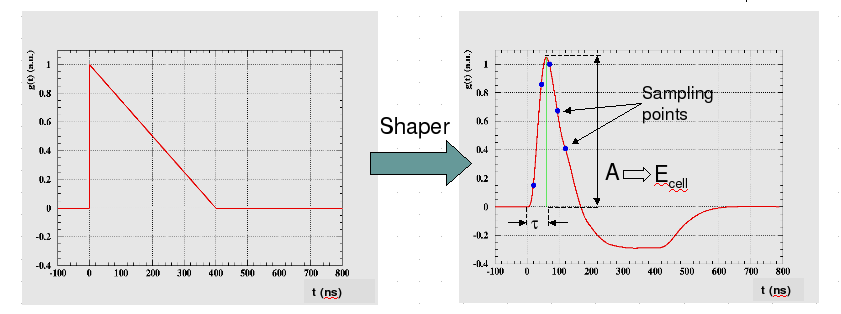
Fig. 1 Right: Ionization (physics) pulse.  Left: Physics pulse at the output of the shaper (see Fig. 4).
Points corresponding to the sampling steps are also shown.

• The energy deposited by the physics pulse is found from the following equation (cf. Fig. 3):

Fig. 2 Finding energy from the physics signal.

• Key question: knowing only the shape of the signal (in ADC counts) can one reconstruct the amplitude A (↔ Ecell) and its position in time τ (while minimizing noise)?

• Isn't the simplest way of calibrating the calorimeter to send particles with known energy and see what we actually reconstruct?

• This, in fact, is done during test beam. However, we cannot test every calo cell this way, only a small fraction in a calo mock-up. The way to do it is to generate pulses using a pulse generator (DAC). These calibration waveforms will simulate the physics pulses.
  

• Thus, calibration involves two types of waveforms: physics pulse resulting from the passage of a particle and calibration (delay) pulses produced by the pulse generator (DAC).

• One needs to be sure that that the generated calibration pulses are equivalent to physics pulses.  Due to the differences in the injection points and differences in shapes, calibration pulses do not faithfully reproduce the physics ones. Thus, we need a way to find a way to go from one type of waveform to the other, i.e. we need to predict the physics pulse from the calibration pulse.

• We use the following formula to find the energy (remember that this is, in a sense, "simulated energy") corresponding to the calibration wave (cf. Fig. 2):
  

  Fig. 3 Finding energy from the calibration signal.

• The sequence to predict a physics pulse from the calibration pulse is the following:

1. Scale the calibration wave so that its max. amplitude is 1 (done for TCM method, below). Alternative method is to scale the amplitude of the physics wave to 1 (done for RTM method, below).  Mphys/Mcali refers the the ratio of the physics to calibration amplitudes, which corrects the for the difference between the calibration and physics signal heights in the TCM.  In the RTM method it is absorbed into the calculation of ADCpeak, thus is not computed explicitly.

2. Find the predicted physics wave. This is done by one of the two complementary methods: TCM and RTM. The real physics waves produced during test beam are either used directly in the prediction (TCM) or, indirectly, to compare it with the predicted wave (RTM).

3. Find the ADCpeak using Optimal Filtering Coefficients (OFC's). Alternative methods of computing the ADCpeak, such as the parabolic interpolation and through Pseudo-Optimal Filtering Coefficients,  also exist.
   

4. Convert ADC to DAC using the ramp relationship.  Σj is given by this formula in the ramp relationship. Rj are second order ramps resulting from the A-to-D conversion.

5. Compute FDAC->μA factor.  FDAC->μA = 76.295 μV/Rinj where Rinj is the value of the injection resistor on the calibration board.

6. Compute FμA->MeV factor.  The meaning of FμA->MeV factor is explained here [PS file].

Calorimeter Calibration Procedure (2004 Test Beam)

Fig. 4 Calibration and physics readout circuit showing the shaper and its effect (top). A more refined representation
of the circuit with the added lumped resistance r  (bottom).

Calibration (Delay) Pulses

• Each calo cell is pulsed N times (typically, 100) with the given input current (DAC value) at a given time delay.

• DAC values are chosen in such a way as not to saturate the ADC. Typically, 16 DAC values were used, making the total number of pulses per cell 16 × 100 = 1600.
  

• DAC = 0 was also used to study the possible effects of the parasitic injected charge (typically around 1 ADC count). See also ramps.
  

• ADC value of each of the N samples is read out and the mean and the RMS values are computed. The averaged waveform for a given DAC value are called Master Waveforms.
  

• The delay is sequentially increased by 1 ns (1.04 ns, to be exact) until the sampling period (25 ns) has been covered.

• The averaged samples are arranged in time according to the delay value.  Thus an averaged profile of samples spaced by 1 ns is obtained, yielding the complete waveform. The total number of samples was 27 and the total waveform was 648 steps long.
  

• The readout pedestal is subtracted.

Physics Pulses

• Electrons and pions of fixed energies (25, 50, 100 GeV) were used to produce physics pulses

• During Test Beam only HIGH and MEDIUM (100 and 10) gains were utilized since the beam energies were never low enough to trigger the LOW gains.